[Webinar] How to Implement Data Contracts: A Shift Left to First-Class Data Products | Register Now
Streaming ETL and Analytics on Confluent with Maritime AIS Data
One of the canonical examples of streaming data is tracking location data over time. Whether it’s ride-sharing vehicles, the position of trains on the rail network, or tracking airplanes waking up your cat, handling the stream of data in real time enables functionality for businesses and their customers in a way that is just not possible in the batch world. Here I’m going to explore another source of streaming data, but away from road and rail—out at sea, with data from ships.
Automatic identification system (AIS) data is broadcast by most ships and can be consumed passively by anyone with a receiver.
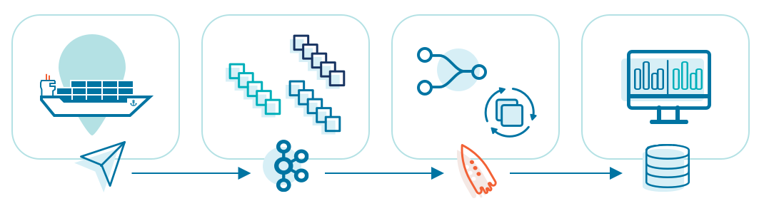
By streaming a feed of AIS data into Apache Kafka®, it’s possible to use it for various purposes, each of which I’m going to explore in more detail.
- Part 1: Analytics and streaming ETL drive both real-time and ad hoc data exploration with a streaming pipeline to cleanse and transform the data.
- Part 2: Stream processing to identify patterns in the data that could suggest certain behaviour.
AIS data
The AIS data source comes from a public feed published under the Norwegian Licence for Open Government Data (NLOD) distributed by the Norwegian Coastal Administration. It covers:
AIS data from all vessels within a coverage area that includes the Norwegian economic zone and the protection zones off Svalbard and Jan Mayen, but with the exception of fishing vessels under 15 meters and recreational vessels under 45 meters
AIS data streams can contain messages of different types. You can check out this great resource on AIS payload interpretation, which explains all the different types and fields associated with each. For example, message type 1 is a Position Report, but it doesn’t include details about the vessel. For that, you need message type 5 (Static and Voyage Related Data).
Often an AIS source is provided as a feed on a TCP/IP port (as in the case of the one used here). As a raw feed, it’s not much to look at:
$ nc 153.44.253.27 5631
\s:2573485,c:1614772291*0C\!BSVDM,1,1,,A,13maq;7000151TNWKWIA3r<v00SI,0*01
\s:2573250,c:1614772291*02\!BSVDO,1,1,,B,402M3hQvDickN0PTuPRwwH7000S:,0*37
!BSVDM,1,1,,A,13o;a20P@K0LIqRSilCa?W4t0<2<,0*19
\s:2573450,c:1614772291*04\!BSVDM,1,1,,B,13m<?c00000tBT`VuBT1anRt00Rs,0*0D
\s:2573145,c:1614772291*05\!BSVDM,1,1,,B,13m91<001IPPnJlQ9HVJppo00<0;,0*33
Fortunately, GPSd provides gpsdecode, which makes a lot more sense of it:
$ nc 153.44.253.27 5631|gpsdecode |jq --unbuffered '.'
{
  "class": "AIS",
  "device": "stdin",
  "type": 1,
  "repeat": 0,
  "mmsi": 259094000,
  "scaled": true,
  "status": 0,
  "status_text": "Under way using engine",
  "turn": 0,
  "speed": 11.4,
  "accuracy": false,
  "lon": 7.085755,
  "lat": 62.656673,
  "course": 179.1,
  "heading": 186,
  "second": 9,
  "maneuver": 0,
  "raim": false,
  "radio": 98618
}
Analytics
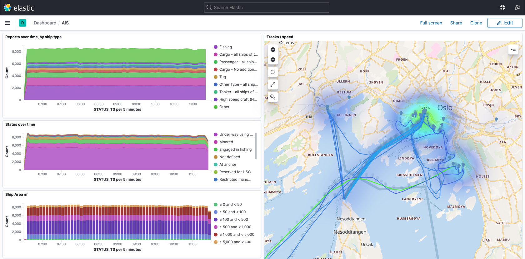
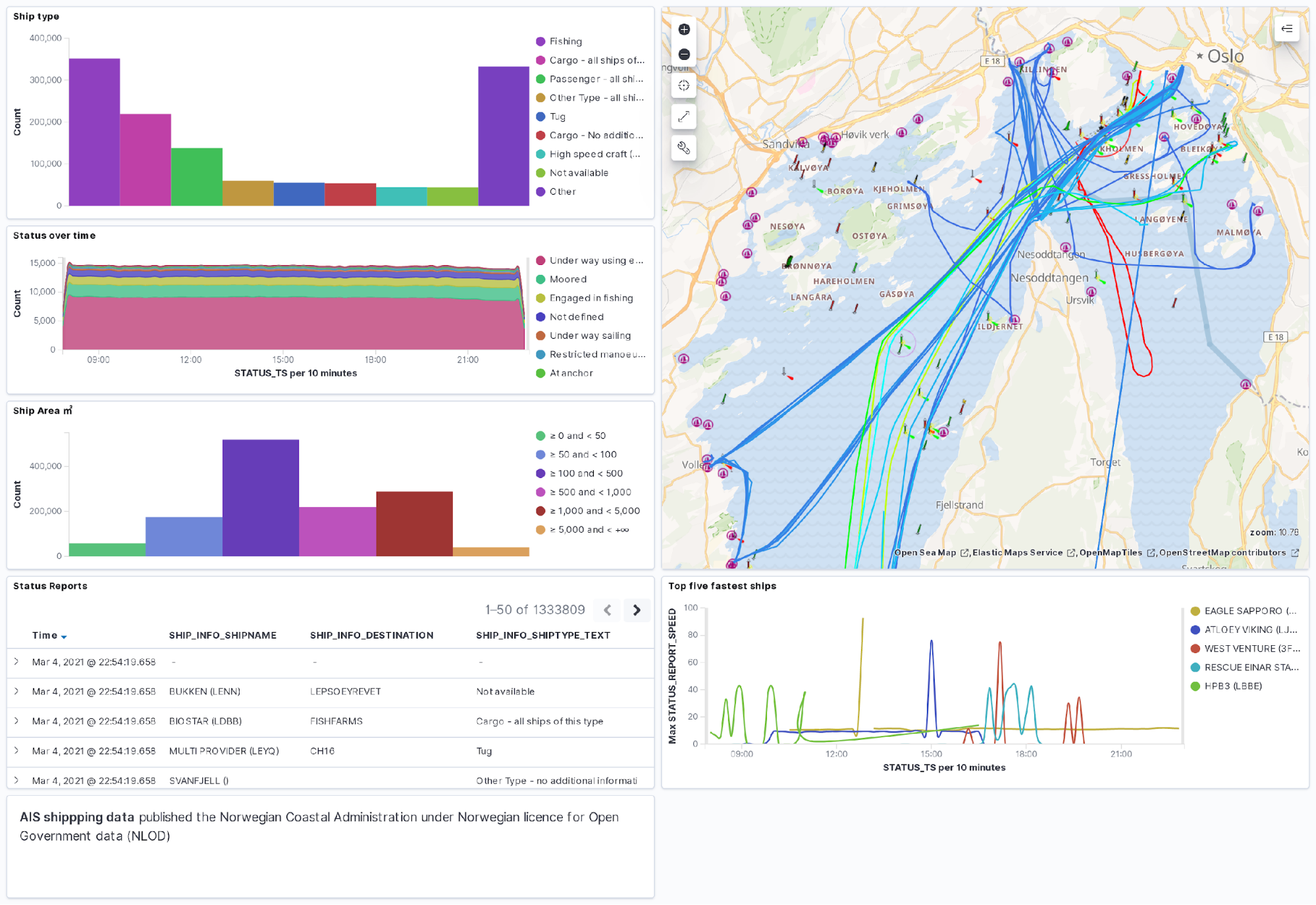
Let’s take a look at the kind of analytics we can easily create from this data, before then taking a step back and walking through how to build it. I’m using Kibana on top of the data held in Elasticsearch with OpenSeaMap tiles added.
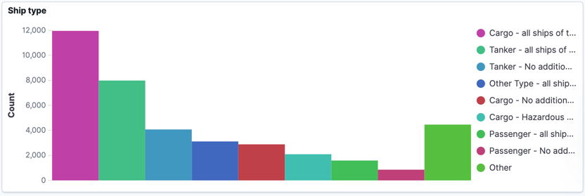
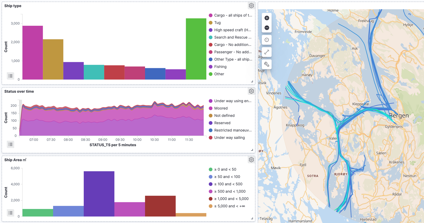
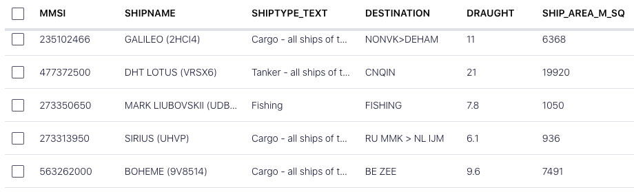
Each ship periodically reports information about itself (AIS message type 5), and we can use that to look at the types of ships:

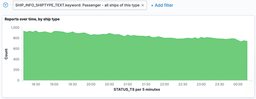
If we filter this just for passenger ships, we can see—as would be expected—fewer reporting in towards the end of the day:
We can also look at other properties of the ships, such as their square area. This is calculated from the AIS data in which the ship’s dimensions are reported:
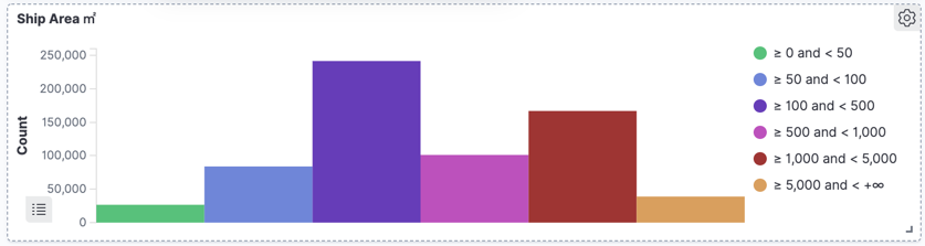
Using Kibana’s filtering, we can drill down into large ships (>5000 ㎡), which unsurprisingly are mostly cargo and tankers:
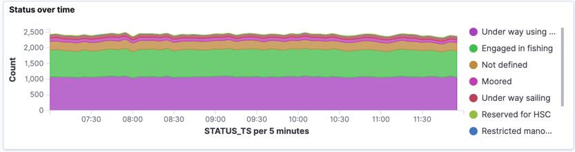
This is pretty interesting, but it only looks at the static data that ships report. What about the continuous stream of data that we get from AIS? This tells us where the ships are and also what they’re reporting as doing. If we filter for ships that report as fishing vessels, we shan’t be too surprised to see that around a third of them are Engaged in fishing:
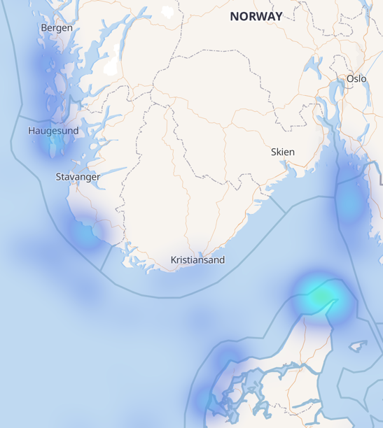
Part of the AIS payload for a status update is the latitude and longitude points reported by the ship, and we can use this to plot the data on a map. Using Kibana’s heatmap option, we can easily see where the most number of fishing vessels are:
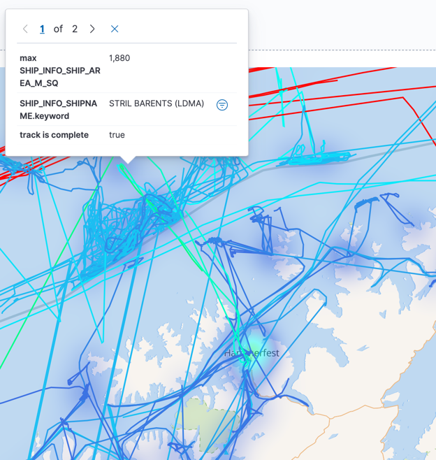
One of the things that I was really interested to see in the version 7.11 release of Kibana was Tracks support in the Map visualisation. By breaking down the data by ship name and callsign, it’s possible to plot the path of each ship:
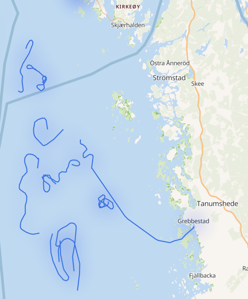
The plot here is just for fishing vessels (as that’s what we’d filtered on previously), but if we open it up to all ships, but vary the track colour based on the size of the ship, we can see patterns starting to form around shipping routes and the different ships using them:
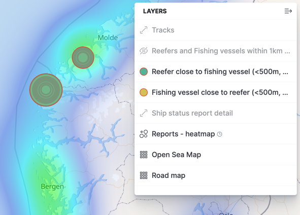
Using the map filtering option, you can draw a region on which to filter the data and examine aggregate information about the ships within it. Here’s everything that’s happening within ~15 km of the city of Bergen, including the associated ship types, activities, and sizes.
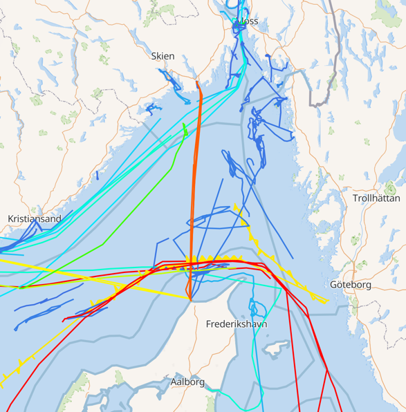
As well as looking at the data in aggregate, you can drill all the way down. I found it fascinating to look at all the shipping activities and then be able to look at a particular vessel. Starting with the map view, you may spot a track that you’re interested in. Here I’ve seen a larger ship and want to know more about it, so click on the track and then the filter button next to the ship’s name.
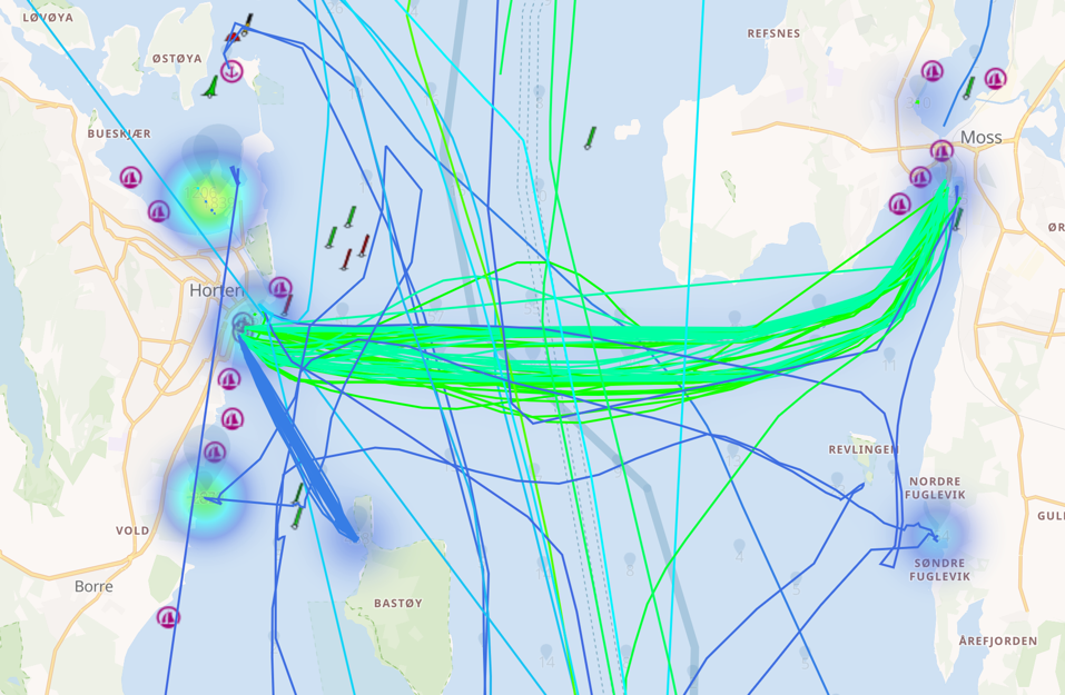
From that, we can now see what it was doing over time:
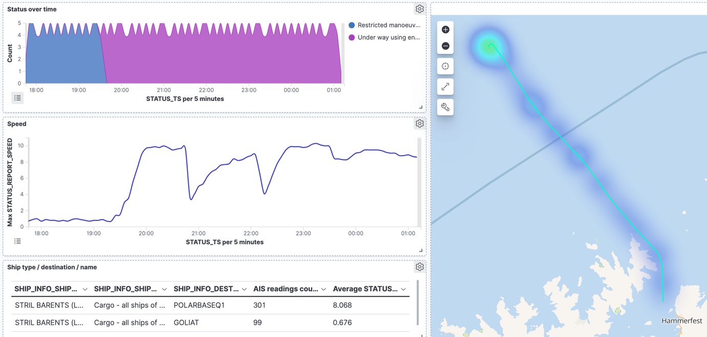
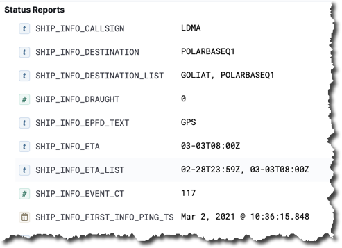
And view individual status reports:
So that’s what we can do; but let’s take a look now at exactly how. As a streaming ETL data pipeline it is a relatively simple one but with some interesting tricks needed along the way…
Streaming ETL – Extract
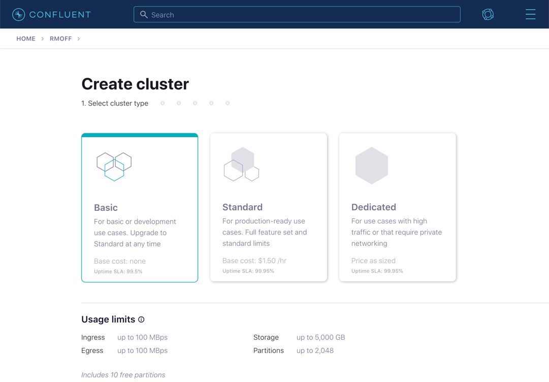
I built all this on Confluent Cloud, so first off, I provisioned myself a cluster:
With API keys in hand, I created a target topic into which to stream the source AIS data:
$ ccloud kafka topic create ais
Created topic "is".
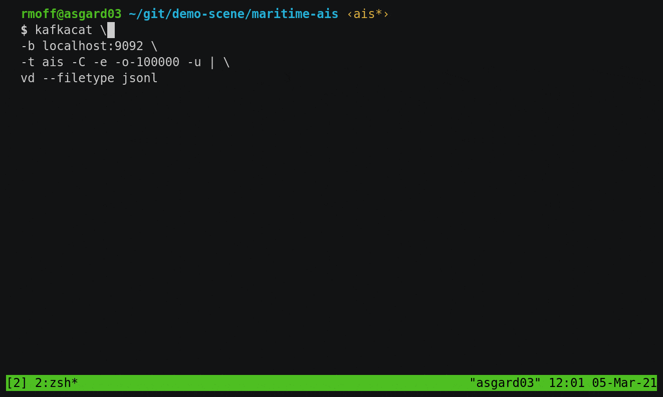
As mentioned above, the raw AIS data can be parsed by gpsdecode to put it into a structured form. From here, I used kafkacat to write it to my Kafka topic. I wrapped this in a Docker container (piggybacking on the existing kafkacat image) to make it self-contained and deployable in the cloud.
$ docker run --rm -t --entrypoint /bin/sh edenhill/kafkacat:1.6.0 -c '
  # Install stuff
$ apk add gpsd gpsd-clients

$ nc 153.44.253.27 5631 | \
  gpsdecode | \
  kafkacat \
    -X security.protocol=SASL_SSL -X sasl.mechanisms=PLAIN \
    -X ssl.ca.location=./etc/ssl/cert.pem -X api.version.request=true \
    -b BROKER.gcp.confluent.cloud:9092 \
    -X sasl.username="API_USER" \
    -X sasl.password="API_PASSWORD" \
    -t ais -P
'
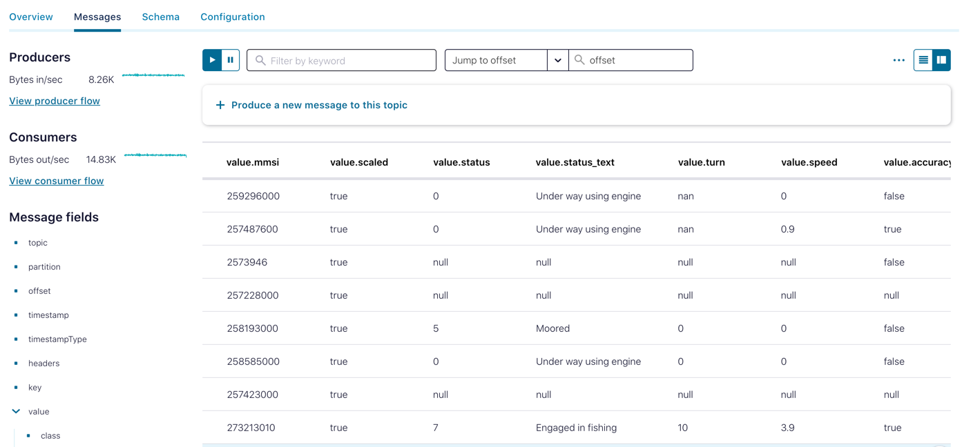
This gave me a stream of data into the ais topic at a rate of around 8 KB/sec. (not really touching the sides of the 100 MB/sec. limit on the lowest-level Confluent Cloud cluster spec).
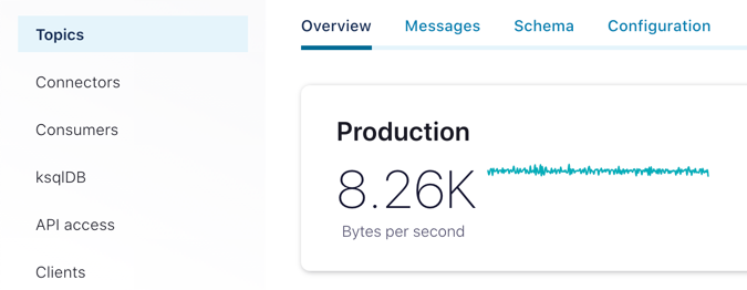
The gpsdecode tool writes the messages out as JSON, which can be inspected with the topic viewer:
Streaming ETL – Transform
With the data streaming in, next up is taking this single stream of events and transforming it into something easily usable. The tool I used for transforming the stream of data was ksqlDB. This lets me use SQL to describe the stream processing that I want to apply to the data.
The raw stream
The first step in ksqlDB was to dump a sample of the topic just to check what we were working with:
ksql> PRINT ais LIMIT 5;
Key format: ¯\_(ツ)_/¯ - no data processed
Value format: JSON or KAFKA_STRING
rowtime: 2021/02/25 10:50:06.934 Z, key: , value: {"class":"AIS","device":"stdin","type":3,"repeat":0,"mmsi":257124880,"scaled":true,"status":15,"status_text":"Not defined","turn":0,, partition: 0ccuracy":false,"lon":11.257358,"lat":64.902517,"course":85.0,"heading":225,"second":2,"maneuver":0,"raim":false,"radio":25283}
rowtime: 2021/02/25 10:50:06.934 Z, key: , value: {"class":"AIS","device":"stdin","type":1,"repeat":0,"mmsi":257045680,"scaled":true,"status":0,"status_text":"Under way using engine", partition: 0"speed":0.3,"accuracy":true,"lon":16.725387,"lat":68.939000,"course":65.7,"heading":511,"second":5,"maneuver":0,"raim":true,"radio":52}
rowtime: 2021/02/25 10:50:06.934 Z, key: , value: {"class":"AIS","device":"stdin","type":5,"repeat":0,"mmsi":259421000,"scaled":true,"imo":9175030,"ais_version":0,"callsign":"LIPZ","shipname":"ROALDNES","shiptype":30,"shiptype_text":"Fishing","to_bow":10,"to_stern":24,"to_port":5,"to_starboard":5,"epfd":1,"epfd_text":"GPS","eta":"01-16T14:00Z","draught":6.3,"destinati, partition: 0,"dte":0}
rowtime: 2021/02/25 10:50:06.934 Z, key: , value: {"class":"AIS","device":"stdin","type":3,"repeat":0,"mmsi":257039700,"scaled":true,"status":5,"status_text":"Moored","turn":0,"speed, partition: 0y":false,"lon":12.273450,"lat":65.998892,"course":188.6,"heading":36,"second":5,"maneuver":0,"raim":false,"radio":0}
rowtime: 2021/02/25 10:50:06.934 Z, key: , value: {"class":"AIS","device":"stdin","type":5,"repeat":0,"mmsi":257956500,"scaled":true,"imo":0,"ais_version":2,"callsign":"LG9456","shipname":"FROY MULTI","shiptype":0,"shiptype_text":"Not available","to_bow":3,"to_stern":12,"to_port":7,"to_starboard":5,"epfd":1,"epfd_text":"GPS","eta":"00-00T24:60Z","draught":0.0,"destina, partition: 0:0}
Topic printing ceased
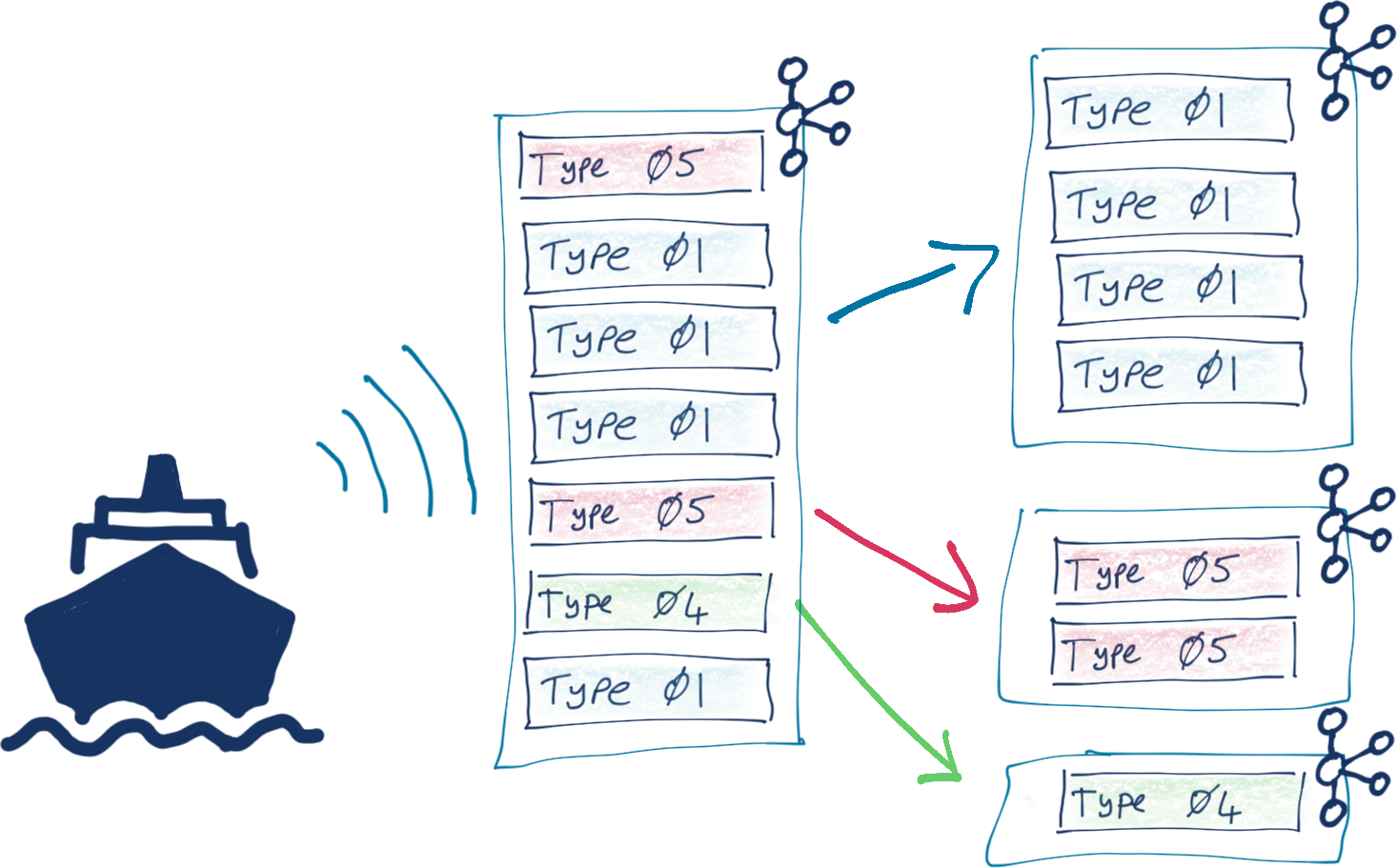
AIS data is broadcast as a single stream of messages of different types. Each message type has its own set of fields, along with some common ones.
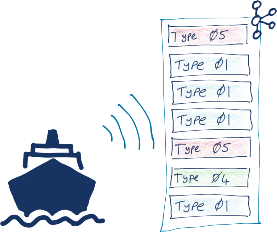
I used a little bit of command line magic to do a quick inspection on a sample of the data to see how many messages of different types I had. Around 75% were position reports, 15% ship information, and the remainder was a mix of other messages.
ksqlDB can be used to split streams of data based on characteristics of the data, and that’s what we needed to do here so that we’d end up with a dedicated stream of messages for each logical type or group of AIS messages. To do any processing with ksqlDB, you need a schema declared on the data (the source data is just lumps of JSON strings without explicit schema). Because there’s a mix of message types (and thus schemas) in the single stream, it’s hard to declare the schema in its entirety upfront, so we use a little trick here to map the first ksqlDB stream. By specifying the serialisation type as KAFKA, we can delay having to declare the schema but still access fields in the data when we need to for the predicate in splitting the stream:
CREATE STREAM AIS_RAW (MSG VARCHAR) WITH (KAFKA_TOPIC='ais', FORMAT='KAFKA');
This declares a stream on the existing ais topic with a single field that we’ve arbitrarily called MSG. The trick is that we’re using the KAFKA format. If we specified it as JSON (as one may reasonably expect, it being JSON data) then there’d have to be a common root field for us to map, which there isn’t.
With a stream declared, we can query it and check that it’s working. The result is pretty much the same as dumping the data with PRINT, but we’re validating now that ksqlDB is happy reading the data:
ksql> SELECT * FROM AIS_RAW EMIT CHANGES LIMIT 5;
+------------------------------------------------------------------------------------------------------------------------------------------------------------------------------------------+
|MSG                                                                                                                                                                                       |
+------------------------------------------------------------------------------------------------------------------------------------------------------------------------------------------+
|{"class":"AIS","device":"stdin","type":3,"repeat":0,"mmsi":259589000,"scaled":true,"status":0,"status_text":"Under way using engine","turn":0,"speed":11.6,"accuracy":false,"lon":11.60895|
|{"class":"AIS","device":"stdin","type":3,"repeat":0,"mmsi":257499000,"scaled":true,"status":5,"status_text":"Moored","turn":0,"speed":0.0,"accuracy":false,"lon":6.447663,"lat":62.593768,|
|{"class":"AIS","device":"stdin","type":1,"repeat":0,"mmsi":259625000,"scaled":true,"status":0,"status_text":"Under way using engine","turn":"nan","speed":0.0,"accuracy":true,"lon":16.542|
|{"class":"AIS","device":"stdin","type":3,"repeat":0,"mmsi":257334400,"scaled":true,"status":5,"status_text":"Moored","turn":0,"speed":0.0,"accuracy":false,"lon":7.732775,"lat":63.113140,|
|{"class":"AIS","device":"stdin","type":5,"repeat":0,"mmsi":257628580,"scaled":true,"imo":0,"ais_version":2,"callsign":"LJ8162","shipname":"MORVIL","shiptype":37,"shiptype_text":"Pleasure|
Limit Reached
Query terminated
Now comes the schema bit. MSG holds the full JSON payload, and we can use EXTRACTJSONFIELD to, as the name suggests, extract JSON fields:
ksql> SELECT EXTRACTJSONFIELD(msg,'$.type') AS MSG_TYPE FROM AIS_RAW EMIT CHANGES LIMIT 5;
+--------------+
|MSG_TYPE      |
+--------------+
|1             |
|1             |
|3             |
|5             |
|1             |
Limit Reached
Query terminated
As shown above, we can set the name of fields that we create (using AS), and we can also CAST data types using other functions, such as TIMESTAMPTOSTRING, as well as use the extracted type field as a predicate:
ksql> SELECT TIMESTAMPTOSTRING(ROWTIME,'yyyy-MM-dd HH:mm:ss','Europe/London') AS TS,
             CAST(EXTRACTJSONFIELD(msg,'$.type') AS INT)                      AS MSG_TYPE,
             CAST(EXTRACTJSONFIELD(msg,'$.status_text') AS VARCHAR)           AS STATUS_TEXT
        FROM AIS_RAW
       WHERE EXTRACTJSONFIELD(msg,'$.type') = '1'
       EMIT CHANGES;

+--------------------+----------+-----------------------+
|TS                  |MSG_TYPE  |STATUS_TEXT            |
+--------------------+----------+-----------------------+
|2021-02-25 10:50:06 |1         |Under way using engine |
|2021-02-25 10:50:09 |1         |Engaged in fishing     |
|2021-02-25 10:50:11 |1         |Not defined            |
|2021-02-25 10:50:17 |1         |Under way using engine |
Based on this, we can populate new dedicated streams just for particular entities with a full schema defined. This is done using the CREATE STREAM…AS SELECT (CSAS) syntax, which writes to a new stream with the continuous results of the declared SELECT statement (which is where the transformations take place). By setting the offset back to earliest, we can process all existing data held on the topic as well as every new message as it arrives. The data is written as Avro (which stores the schema in the Confluent Schema Registry), and the message partitioning key is set with PARTITION BY to the unique identifier of the vessel (MMSI).
You can find the full SQL declarations in the repository, but as a general pattern, they look something like this:
- Ship position reports (type 1, 2, or 3 messages):
CREATE OR REPLACE STREAM AIS_MSG_TYPE_1_2_3 WITH (FORMAT='AVRO') AS SELECT CAST(EXTRACTJSONFIELD(msg,'$.type') AS INT) AS msg_type, CAST(EXTRACTJSONFIELD(msg,'$.mmsi') AS VARCHAR) AS mmsi, CAST(EXTRACTJSONFIELD(msg,'$.status_text') AS VARCHAR) AS status_text, CAST(EXTRACTJSONFIELD(msg,'$.speed') AS DOUBLE) AS speed, CAST(EXTRACTJSONFIELD(msg,'$.course') AS DOUBLE) AS course, CAST(EXTRACTJSONFIELD(msg,'$.heading') AS INT) AS heading FROM AIS_RAW WHERE EXTRACTJSONFIELD(msg,'$.type') IN ('1' ,'2' ,'3' ,'18' ,'27') PARTITION BY CAST(EXTRACTJSONFIELD(msg,'$.mmsi') AS VARCHAR); - Ship and voyage data (type 5 messages):
CREATE OR REPLACE STREAM AIS_MSG_TYPE_5 WITH (FORMAT='AVRO')          AS
  SELECT  CAST(EXTRACTJSONFIELD(msg,'$.type') AS INT)                 AS msg_type,
          CAST(EXTRACTJSONFIELD(msg,'$.mmsi') AS VARCHAR)             AS mmsi,
          CAST(EXTRACTJSONFIELD(msg,'$.callsign') AS VARCHAR)         AS callsign,
          CAST(EXTRACTJSONFIELD(msg,'$.shipname') AS VARCHAR)         AS shipname_raw,
          CONCAT(CAST(EXTRACTJSONFIELD(msg,'$.shipname') AS VARCHAR),
                 ' (',
                 CAST(EXTRACTJSONFIELD(msg,'$.callsign') AS VARCHAR),
                 ')')                                                 AS shipname,
          CAST(EXTRACTJSONFIELD(msg,'$.shiptype_text') AS VARCHAR)    AS shiptype_text,
          CAST(EXTRACTJSONFIELD(msg,'$.destination') AS VARCHAR)      AS destination
  FROM    AIS_RAW
  WHERE   EXTRACTJSONFIELD(msg,'$.type') = '5'
  PARTITION BY CAST(EXTRACTJSONFIELD(msg,'$.mmsi') AS VARCHAR);
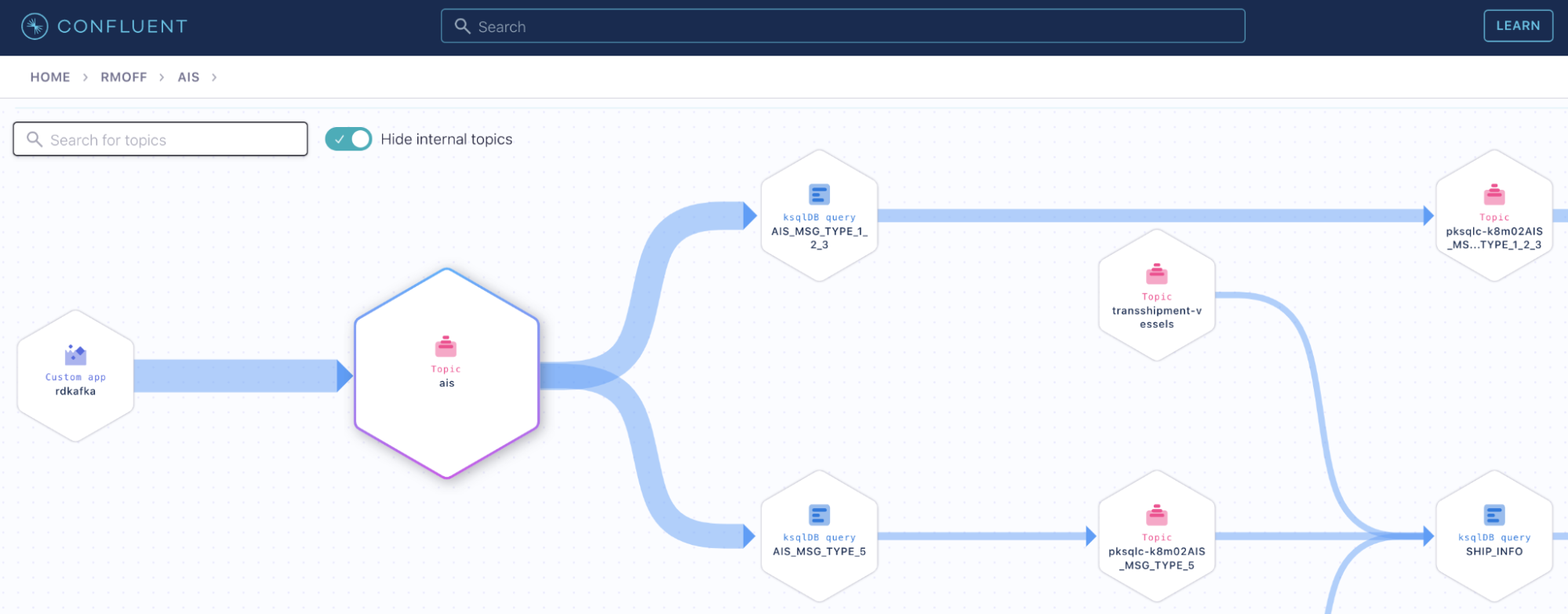
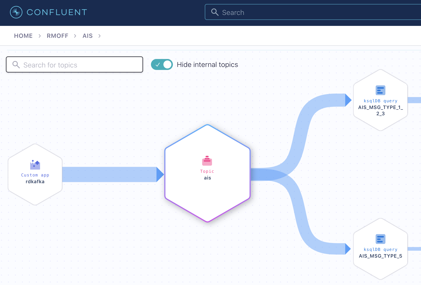
After this, there are now three streams—the original (AIS_RAW) along with streams holding only messages of a certain type:
ksql> SHOW STREAMS;

 Stream Name                    | Kafka Topic                        | Key Format | Value Format | Windowed
------------------------------------------------------------------------------------------------------------
 AIS_MSG_TYPE_1_2_3             | AIS_MSG_TYPE_1_2_3                 | AVRO       | AVRO         | false
 AIS_MSG_TYPE_5                 | AIS_MSG_TYPE_5                     | AVRO       | AVRO         | false
 AIS_RAW                        | ais                                | KAFKA      | KAFKA        | false
Building a lookup table from a stream of events
The status report messages in the stream AIS_MSG_TYPE_1_2_3 are nice, simple events. A ship was here, and then it was there, and then it was over there.
ksql> SELECT MMSI, STATUS_TEXT, LON, LAT
        FROM AIS_MSG_TYPE_1_2_3
       WHERE MMSI = '257293400'
       EMIT CHANGES;
+----------+-----------------------+----------+----------+
|MMSI      |STATUS_TEXT            |LON       |LAT       |
+----------+-----------------------+----------+----------+
|257293400 |Under way using engine |15.995308 |68.417305 |
|257293400 |Under way using engine |15.995307 |68.417282 |
|257293400 |Under way using engine |15.995288 |68.417288 |
…
But let’s now think about the type 5 messages, which describe the ship’s characteristics. In the old world of batch data, this would be a straight-up “dimension” or “lookup” table. What does that look like in a streaming world?
Well, it actually looks pretty similar. It’s still a table! The important thing here is that the key is crucial. A ksqlDB table maintains the latest value for each key based on the messages in a Kafka topic. Consider this stream of messages on the AIS_MSG_TYPE_5 stream that we have built:
ksql> SELECT TIMESTAMPTOSTRING(ROWTIME,'HH:mm:ss','Europe/Oslo') AS TS,
             MMSI,
             SHIPNAME,
             DRAUGHT,
             DESTINATION
        FROM AIS_MSG_TYPE_5
       WHERE MMSI = '255805587'
       EMIT CHANGES;
+---------+-----------+------------------+--------+------------+
|TS       |MMSI       |SHIPNAME          |DRAUGHT |DESTINATION |
+---------+-----------+------------------+--------+------------+
|11:17:17 |255805587  |NCL AVEROY (CQHL) |7.5     |SVELGEN     |
|12:47:26 |255805587  |NCL AVEROY (CQHL) |7.5     |SVELGEN     |
|13:06:27 |255805587  |NCL AVEROY (CQHL) |7.5     |MALOY       |
|13:13:43 |255805587  |NCL AVEROY (CQHL) |7.5     |FLORO       |
…
Here we can see that some attributes are unchanged (the ship’s name, its callsign, and its draught), which we would expect, whilst others (its reported destination) can vary over time. We model this stream of events as a table, taking the unique identifier (the MMSI) as the key (GROUP BY):
CREATE TABLE SHIP_INFO AS
  SELECT MMSI,
        MAX(ROWTIME) AS LAST_INFO_PING_TS,
        LATEST_BY_OFFSET(SHIPNAME) AS SHIPNAME,
        LATEST_BY_OFFSET(DRAUGHT) AS DRAUGHT,
        LATEST_BY_OFFSET(DESTINATION) AS DESTINATION
    FROM AIS_MSG_TYPE_5
  GROUP BY MMSI
  EMIT CHANGES;
When we query this table, at first, it will show the state at that point in time:
SELECT MMSI,
       TIMESTAMPTOSTRING(LAST_INFO_PING_TS,'HH:mm:ss','Europe/London') AS LAST_INFO_PING_TS,
       SHIPNAME,DRAUGHT, DESTINATION FROM SHIP_INFO WHERE MMSI = '255805587';

+----------+------------------+------------------+--------+------------+
|MMSI      |LAST_INFO_PING_TS |SHIPNAME          |DRAUGHT |DESTINATION |
+----------+------------------+------------------+--------+------------+
|255805587 |11:17:17          |NCL AVEROY (CQHL) |7.5     |SVELGEN     |
+----------+------------------+------------------+--------+------------+
As new messages arrive on the underlying source topic, the value for the key (MMSI) changes, and so does the state of the table:
+----------+------------------+------------------+--------+------------+
|MMSI      |LAST_INFO_PING_TS |SHIPNAME          |DRAUGHT |DESTINATION |
+----------+------------------+------------------+--------+------------+
|255805587 |13:06:27          |NCL AVEROY (CQHL) |7.5     |MALOY       |
+----------+------------------+------------------+--------+------------+
This table is held as a materialised view within ksqlDB and also as a Kafka topic. This means that we can do several things with it:
- Join it to a stream of events (“facts”), as we will see shortly
- Query the state from an external application using a pull query from a Java client or other REST API client
- Push the state to an external data store such as a database
Joining ship movements to ship information
To do useful things with the data, we want to join messages from the same original stream to each other. We want to denormalise the information provided in one message about a ship’s movements to additional information provided in another message about the ship’s characteristics.
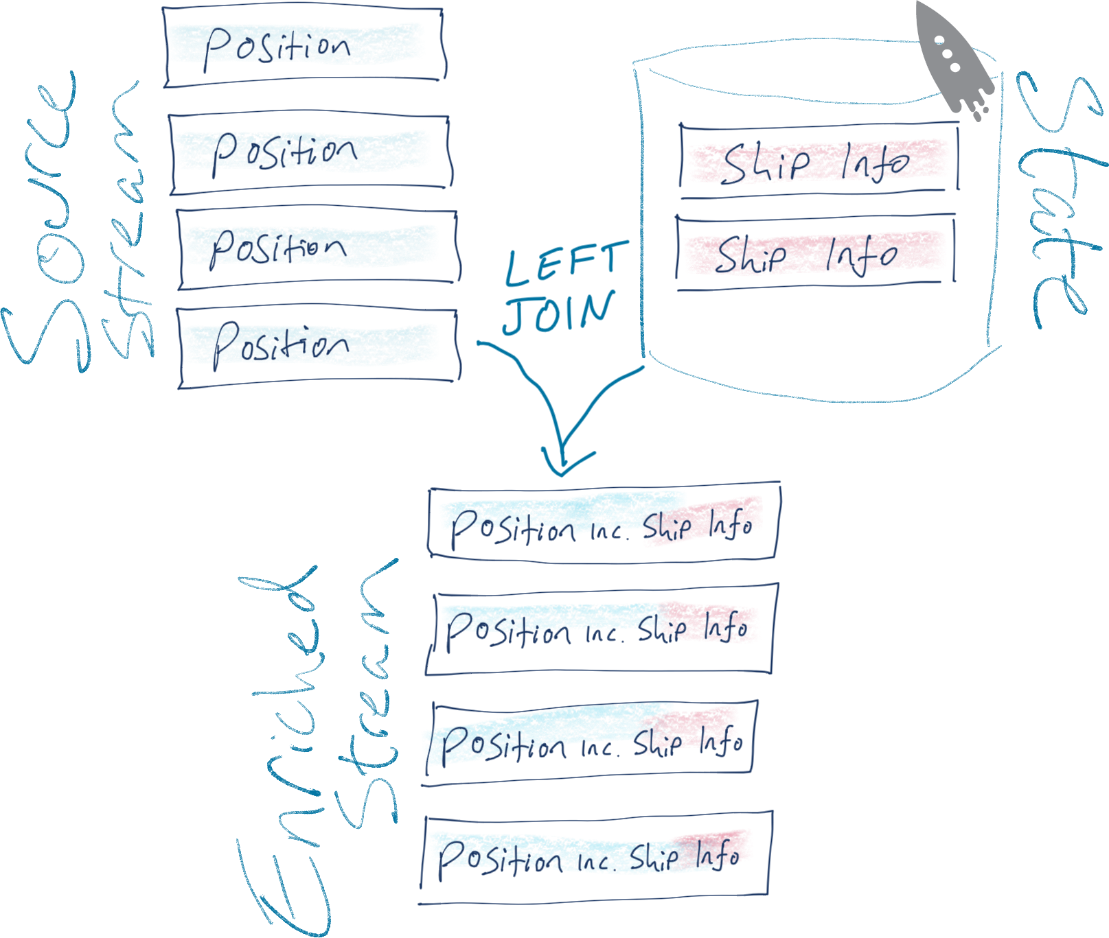
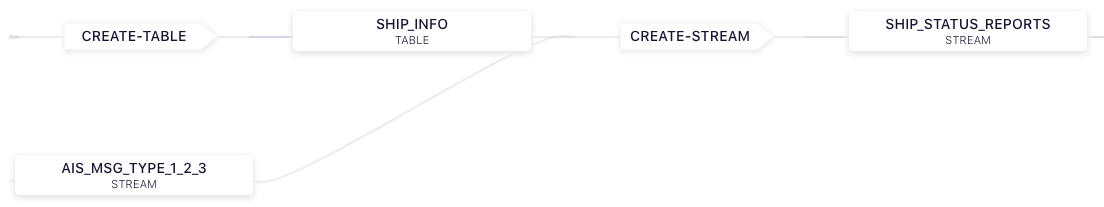
As discussed above, the ship’s characteristics is modelled as a ksqlDB table, which is then joined to the stream of ship position updates, thus:
CREATE STREAM SHIP_STATUS_REPORTS WITH
  (KAFKA_TOPIC='SHIP_STATUS_REPORTS_V00') AS
SELECT STATUS_REPORT.ROWTIME AS STATUS_TS,
       STATUS_REPORT.*,
       SHIP_INFO.*
FROM  AIS_MSG_TYPE_1_2_3 STATUS_REPORT
      LEFT JOIN SHIP_INFO SHIP_INFO
        ON STATUS_REPORT.MMSI = SHIP_INFO.MMSI
;
This writes to a new Kafka topic every message from the source stream (AIS_MSG_TYPE_1_2_3) enriched with, when found, the information about the ship (that originally came from the AIS_MSG_TYPE_5 stream), then modelled into a table holding state. The name for the Kafka topic is inherited from the stream name, unless explicitly defined (as in the example above).
You can also do stream-to-stream joins in ksqlDB, and we’ll see a good use for those later on.
With the joined data stream, we can now see for a given ship every movement along with information about the ship itself:
ksql> SELECT TIMESTAMPTOSTRING(STATUS_TS,'HH:mm:ss','Europe/Oslo') AS STATUS_TS,
             SHIP_LOCATION,
             STATUS_REPORT_STATUS_TEXT,
             SHIP_INFO_SHIPNAME,
             SHIP_INFO_DRAUGHT,
             SHIP_INFO_DESTINATION_LIST
        FROM SHIP_STATUS_REPORTS
       WHERE SHIP_INFO_MMSI = '255805587'
       EMIT CHANGES;
+-----------+--------------------------------+---------------------------+---------------------+-------------------+----------------------+
|STATUS_TS  |SHIP_LOCATION                   |STATUS_REPORT_STATUS_TEXT  |SHIP_INFO_SHIPNAME   |SHIP_INFO_DRAUGHT  |SHIP_INFO_DESTINATION |
+-----------+--------------------------------+---------------------------+---------------------+-------------------+----------------------+
|11:37:47   |{lat=61.773223, lon=5.294023}   |Moored                     |NCL AVEROY (CQHL)    |7.5                |[SVELGEN]             |
[…]
|17:16:45   |{lat=61.939807, lon=5.143242}   |Under way using engine     |NCL AVEROY (CQHL)    |7.5                |[FLORO]               |
[…]
|23:05:25   |{lat=62.468148, lon=6.137387}   |Under way using engine     |NCL AVEROY (CQHL)    |8.1                |[ALESUND]             |
[…]
|23:11:04   |{lat=62.468122, lon=6.13745}    |Under way using engine     |NCL AVEROY (CQHL)    |8.1                |[ALESUND]             |
[…]
|23:35:47   |{lat=62.468125, lon=6.137473}   |Moored                     |NCL AVEROY (CQHL)    |8.1                |[ALESUND]             |
[…]
If you get really curious about a particular ship, you can even go and look up more information about it over on MarineTraffic.
The output of this is a Kafka topic, and we’ll see shortly what we did with it next. First though, I’d like to discuss some of the nitty-gritty of the streaming ETL work, illustrating the kind of real-world problems that data engineers encounter and can solve with ksqlDB.
Cleaning up the data’s latitude and longitude values
Some of the location values reported in the feed turned out to be a bit…unlikely.
{
  "type": 1,
  "repeat": 0,
  "mmsi": 257565600,
  "status_text": "Under way using engine",
  "lon": 181.000000,
  "lat": 91.000000,
  "course": 360.0,
  "heading": 511
  …
}
The latitude and longitude are reported as 91 and 181, respectively, which is nonsensical (the valid limits are -90/90 and -180/180).
Because we’re going to be doing work with these location values downstream, we should clean this data up. We have different options available to us. If the data is just offset incorrectly, then we could recalculate it, but here we’re going to assume that it’s junk and null it out.
Let’s test that this is going to work. First up, we’ll dump a bunch of messages and eyeball them to identify ships by their unique code (MMSI), for a couple with valid location readings and one with the dodgy values:
SELECT TIMESTAMPTOSTRING(ROWTIME,'yyyy-MM-dd HH:mm:ss','Europe/Oslo') AS TS,
       EXTRACTJSONFIELD(msg,'$.mmsi'),
       EXTRACTJSONFIELD(msg,'$.lon'),
       EXTRACTJSONFIELD(msg,'$.lat')
  FROM AIS_RAW
  EMIT CHANGES LIMIT 500;

+--------------------+--------------------+--------------------+--------------------+
|TS                  |KSQL_COL_0          |KSQL_COL_1          |KSQL_COL_2          |
+--------------------+--------------------+--------------------+--------------------+
|2021-02-25 10:50:06 |257124880           |11.257358           |64.902517           |
|2021-02-25 10:50:06 |257045680           |16.725387           |68.939000           |
…
…
…
|2021-02-25 10:50:13 |257014400           |181.000000          |91.000000           |
|2021-02-25 10:50:13 |273322840           |32.357117           |70.427183           |
Now let’s use those identifiers (257124880, 257045680, and 257014400) to sample records just for these ships, using a WHERE clause with an IN predicate:
SELECT TIMESTAMPTOSTRING(ROWTIME,'yyyy-MM-dd HH:mm:ss','Europe/Oslo') AS TS,
       EXTRACTJSONFIELD(msg,'$.mmsi'),
       EXTRACTJSONFIELD(msg,'$.lon'),
       EXTRACTJSONFIELD(msg,'$.lat')
  FROM AIS_RAW
  WHERE EXTRACTJSONFIELD(msg,'$.mmsi') IN (257124880, 257045680, 257014400)
  EMIT CHANGES LIMIT 3;

+--------------------+--------------------+--------------------+--------------------+
|TS                  |KSQL_COL_0          |KSQL_COL_1          |KSQL_COL_2          |
+--------------------+--------------------+--------------------+--------------------+
|2021-02-25 10:50:06 |257124880           |11.257358           |64.902517           |
|2021-02-25 10:50:06 |257045680           |16.725387           |68.939000           |
|2021-02-25 10:50:13 |257014400           |181.000000          |91.000000           |
Limit Reached
Query terminated
Now we can transform the source lat/lon fields to their target format (DOUBLE) but use a CASE to handle these out of range values. Note that if either lat or lon is invalid, we store a NULL for both. We’ll test it using the same messages as above.
SELECT TIMESTAMPTOSTRING(ROWTIME,'yyyy-MM-dd HH:mm:ss','Europe/Oslo') AS TS,
       EXTRACTJSONFIELD(msg,'$.mmsi') AS MMSI,
       EXTRACTJSONFIELD(msg,'$.lat') AS RAW_LAT,
       EXTRACTJSONFIELD(msg,'$.lon') AS RAW_LON,
       CASE
         WHEN (   CAST(EXTRACTJSONFIELD(msg,'$.lon') AS DOUBLE) >  180
               OR CAST(EXTRACTJSONFIELD(msg,'$.lon') AS DOUBLE) < -180 OR CAST(EXTRACTJSONFIELD(msg,'$.lat') AS DOUBLE) >   90
               OR CAST(EXTRACTJSONFIELD(msg,'$.lat') AS DOUBLE) < - 90) THEN CAST(NULL AS DOUBLE) ELSE CAST(EXTRACTJSONFIELD(msg,'$.lon') AS DOUBLE) END AS lon, CASE WHEN ( CAST(EXTRACTJSONFIELD(msg,'$.lon') AS DOUBLE) >  180
               OR CAST(EXTRACTJSONFIELD(msg,'$.lon') AS DOUBLE) < -180 OR CAST(EXTRACTJSONFIELD(msg,'$.lat') AS DOUBLE) >   90
               OR CAST(EXTRACTJSONFIELD(msg,'$.lat') AS DOUBLE) < - 90) THEN CAST(NULL AS DOUBLE)
         ELSE CAST(EXTRACTJSONFIELD(msg,'$.lat') AS DOUBLE) END AS lat,
   FROM AIS_RAW
  WHERE EXTRACTJSONFIELD(msg,'$.mmsi') IN (257124880, 257045680, 257014400)
  EMIT CHANGES LIMIT 3;
+-------------------+-----------+-----------+------------+----------+----------+
|TS                 |MMSI       |RAW_LAT    |RAW_LON     |LAT       |LON       |
+-------------------+-----------+-----------+------------+----------+----------+
|2021-02-25 10:50:06|257124880  |64.902517  |11.257358   |64.902517 |11.257358 |
|2021-02-25 10:50:06|257045680  |68.939000  |16.725387   |68.939    |16.725387 |
|2021-02-25 10:50:13|257014400  |91.000000  |181.000000  |null      |null      |
Limit Reached
Query terminated
Creating a location object
Because latitude and longitude aren’t two fields in isolation but actually a pair of values that exist together and don’t make much sense individually, we’re going to transform them into a nested object in the schema. We do this using STRUCT in the SELECT statement and define the fields to nest within it:
STRUCT("lat" := LAT, "lon" := LON)
Note that we use quote marks to force the field names to lowercase, as this is what Elasticsearch needs downstream to recognise the object as a geopoint (if it’s LAT/LON it won’t work—it has to be lat/lon).
We also need to handle the null values that we created in the cleanup process above, which we do using a CASE and IS NULL predicate, which when it evaluates to true builds the necessary null object struct to maintain compatibility with the schema:
WHEN LAT IS NULL OR LON IS NULL THEN
  CAST(NULL AS STRUCT<`lat` DOUBLE, `lon` DOUBLE>)
The full SQL looks like this:
SELECT TIMESTAMPTOSTRING(ROWTIME,'yyyy-MM-dd HH:mm:ss','Europe/Oslo') AS TS,
       MMSI, LAT, LON,
       CASE
         WHEN LAT IS NULL OR LON IS NULL THEN
           CAST(NULL AS STRUCT<`lat` DOUBLE, `lon` DOUBLE>)
         ELSE
           STRUCT("lat" := LAT, "lon" := LON)
       END AS LOCATION
  FROM AIS_MSG_TYPE_1_2_3
 WHERE MMSI IN (257124880, 257045680, 257014400)
 EMIT CHANGES;
+---------------------+-----------+----------+----------+-------------------------------+
|TS                   |MMSI       |LAT       |LON       |LOCATION                       |
+---------------------+-----------+----------+----------+-------------------------------+
|2021-02-25 10:50:06  |257124880  |64.902517 |11.257358 |{lat=64.902517, lon=11.257358} |
|2021-02-25 10:50:06  |257045680  |68.939    |16.725387 |{lat=68.939, lon=16.725387}    |
|2021-02-25 10:50:13  |257014400  |null      |null      |null                           |
…
Uniquely identifying ships
When I plotted the movements of a ship identified by its name alone, I got this:
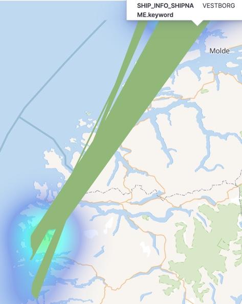
It turns out that ship names are not unique, as can be seen if we query the stream of data and observe the call sign and MMSI:
ksql> SELECT MMSI, CALLSIGN, SHIPNAME FROM SHIP_INFO WHERE SHIPNAME='VESTBORG' EMIT CHANGES;
+-----------+----------+---------+
|MMSI       |CALLSIGN  |SHIPNAME |
+-----------+----------+---------+
|219000035  |OXMC2     |VESTBORG |
|257477000  |LAIQ8     |VESTBORG |
So, we create a compound column using SQL to include the call sign, giving us a field that’s still human readable (unlike MMSI) but now hopefully unique:
ksql> SELECT MMSI, CALLSIGN, SHIPNAME AS SHIPNAME_RAW,
             CONCAT(SHIPNAME,' (',CALLSIGN,')') AS SHIPNAME
        FROM SHIP_INFO SHIPNAME='VESTBORG' EMIT CHANGES;
+----------+---------+-------------+-----------------+
|MMSI      |CALLSIGN |SHIPNAME_RAW |SHIPNAME         |
+----------+---------+-------------+-----------------+
|257477000 |LAIQ8    |VESTBORG     |VESTBORG (LAIQ8) |
|219000035 |OXMC2    |VESTBORG     |VESTBORG (OXMC2) |
Tracking destinations
Looking at the source stream of updates, we can see that the destination can change over time (as would be expected):
ksql> SELECT TIMESTAMPTOSTRING(ROWTIME,'yyyy-MM-dd HH:mm:ss','Europe/London') AS TS, MMSI,
>         SHIPNAME,
>         DESTINATION
>    FROM AIS_MSG_TYPE_5 WHERE MMSI=311411000
>emit changes;
+---------------------+-------------+------------+
|TS                   |SHIPNAME     |DESTINATION |
+---------------------+-------------+------------+
|2021-02-25 09:56:01  |SAMSKIP ICE  |TROMSO      |
…
|2021-02-25 12:38:06  |SAMSKIP ICE  |TROMSO      |
|2021-02-25 12:41:59  |SAMSKIP ICE  |SORTLAND    |
|2021-02-25 12:41:59  |SAMSKIP ICE  |SORTLAND    |
|2021-02-25 13:42:42  |SAMSKIP ICE  |LODINGEN    |
|2021-02-25 13:48:42  |SAMSKIP ICE  |LODINGEN    |
…
We’re building a table that holds the current state of ships, including their current reported destination. It will also be useful to have a full list of the destinations available on the table for direct querying. We can use the COLLECT_SET aggregation for this:
ksql> SELECT TIMESTAMPTOSTRING(LATEST_BY_OFFSET(ROWTIME),'yyyy-MM-dd HH:mm:ss','Europe/London') AS TS,
             MMSI,
             LATEST_BY_OFFSET(SHIPNAME) AS SHIPNAME,
             LATEST_BY_OFFSET(DESTINATION) AS DESTINATION,
             COLLECT_SET(DESTINATION) AS DESTINATIONS
        FROM AIS_MSG_TYPE_5
        WHERE MMSI=311411000
        GROUP BY MMSI
        EMIT CHANGES;
+----------------------+----------------------+----------------------+----------------------+----------------------+
|TS                    |MMSI                  |SHIPNAME              |DESTINATION           |DESTINATIONS          |
+----------------------+----------------------+----------------------+----------------------+----------------------+
|2021-02-25 11:26:05   |311411000             |SAMSKIP ICE           |TROMSO                |[TROMSO]              |
|2021-02-25 14:12:43   |311411000             |SAMSKIP ICE           |LODINGEN              |[TROMSO, SORTLAND, LOD|
|                      |                      |                      |                      |INGEN]
Streaming ETL – Transform recap
I’ve described quite a lot of the pipeline details, hopefully to both flesh out the practical beyond just the theory as well as give some tips and tricks for its use in other applications. To recap on the overall pipeline:
- We’ve modelled the inbound raw stream of AIS data in JSON format into a ksqlDB stream, with no schema to start with
- We split the stream based on message types and applied the relevant schema to each type
- We converted the stream of ship information messages to state by modelling it as a ksqlDB table
- We joined the ship status reports to the ship information table to create an enriched (denormalised) stream of real-time data about ship movements combined with information about that ship
The final result is a real-time feed into a Kafka topic that can then be used for subsequent processing, as described below.
Streaming ETL – Load
Let’s finish off this journey through streaming ETL in action with the final, logical step: load. Load has got such a stodgy batch connotation to it; what we’re building here is streaming ingest into another system. Here I’m using Elasticsearch for analytics. Because the source data exists on a Kafka topic and is retained there, I could easily add in additional targets using the same data.
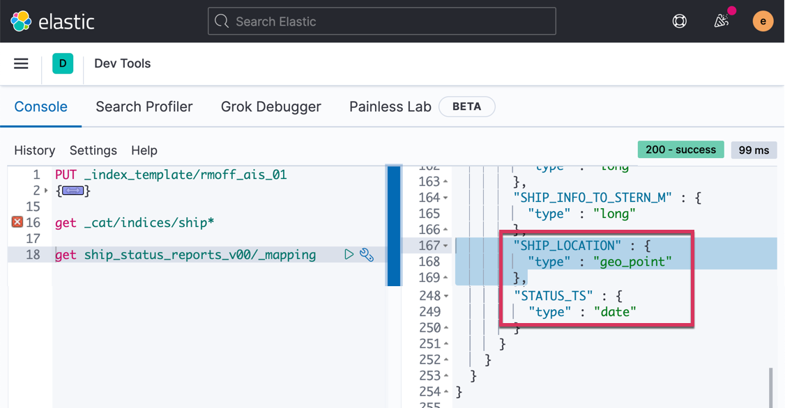
I’m using Elastic Cloud here, which, like Confluent Cloud, provides a fully managed platform and makes my life a whole lot easier. Before we stream the data into Elasticsearch, we need to create an index template to define a couple of important field type mappings. You can do this in Kibana Dev Tools or with the REST API directly:
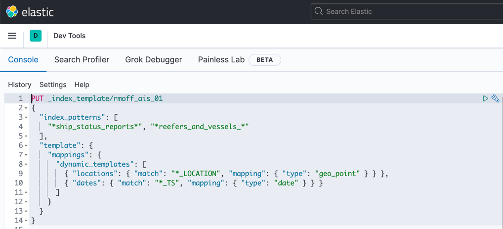
This ensures that any field we send over that ends in _TS is mapped as a date and _LOCATION as a geopoint.
Now we can go and get that ingest running. You can run Kafka Connect yourself to handle integration in and out of Kafka, but because we’ve got all our data in Confluent Cloud, let’s make use of the managed connectors that it provides, including one for Elasticsearch:
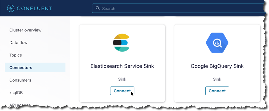
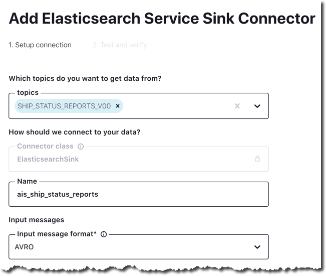
We fill in a few details, including the name of the source topic, location, and credentials for the Elasticsearch cluster:
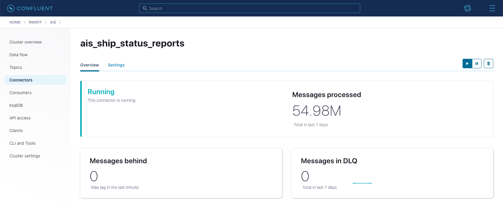
We are now ready to go!
Making sure that the data types have been set in the new Elasticsearch index is important, and we can check that from Kibana Dev Tools again:
With that done, all that remains now is to build our dashboard and analytics in Kibana.
In closing…
It’s pretty neat what we’ve been able to build here with a bit of SQL and some managed cloud services. Check out part 2, in which I show an example of using stream processing to identify the particular behaviour of interest of ships in the AIS data.
You can try Confluent Cloud using code RMOFF200 for $200 off your bill.
If you’d rather run this on premises, you can do that too, using Docker Compose and instructions in the GitHub repo.
Acknowledgments
My huge thanks to Lars Roar Uggerud Dugstad for prompting my curiosity with his question on Stack Overflow, and for all his help in scratching the figurative itch that it prompted!
AIS data distributed by the Norwegian Coastal Administration under Norwegian licence for Open Government data (NLOD).
Datasets distributed by Global Fishing Watch under Creative Commons Attribution-ShareAlike 4.0 International license.
Did you like this blog post? Share it now
Subscribe to the Confluent blog


3 Strategies for Achieving Data Efficiency in Modern Organizations
The efficient management of exponentially growing data is achieved with a multipronged approach based around left-shifted (early-in-the-pipeline) governance and stream processing.


Chopped: AI Edition - Building a Meal Planner
Dinnertime with picky toddlers is chaos, so I built an AI-powered meal planner using event-driven multi-agent systems. With Kafka, Flink, and LangChain, agents handle meal planning, syncing preferences, and optimizing grocery lists. This architecture isn’t just for food, it can tackle any workflow.