New in Confluent Cloud: Making Data & Pipelines Accessible for AI-Ready Streaming | Learn More
How to Tune RocksDB for Your Kafka Streams Application
Apache Kafka ships with Kafka Streams, a powerful yet lightweight client library for Java and Scala to implement highly scalable and elastic applications and microservices that process and analyze data stored in Kafka. A Kafka Streams application can perform stateless operations like maps and filters as well as stateful operations like windowed joins and aggregations on incoming data records.
For stateful operations, Kafka Streams uses local state stores that are made fault-tolerant by associated changelog topics stored in Kafka. For these state stores, Kafka Streams uses RocksDB as its default storage to maintain local state on a computing node (think: a container that runs one instance of your distributed application). RocksDB is a highly adaptable, embeddable, and persistent key-value store that was originally built by the Engineering team at Facebook. Many companies use RocksDB in their infrastructure to get high performance to serve data. Kafka Streams configures RocksDB to deliver a write-optimized state store.
This blog post will cover key concepts that show how Kafka Streams uses RocksDB to maintain its state and how you can tune RocksDB for Kafka Streams’ state stores. We’ll first explain the basics around Kafka Streams and how it uses state stores. Then, we‘ll provide an overview about RocksDB, including the two most used compaction styles, level compaction and universal compaction. Once we understand the foundational principles, we’ll deep dive into operational issues that you may encounter when you operate your Kafka Streams application with RocksDB state stores, and most importantly how you can tune RocksDB to overcome those issues.
Kafka Streams basics
Kafka Streams defines its computational logic through a so-called topology. A topology consists of processors connected by streams. A processor executes its logic on a stream record by record.
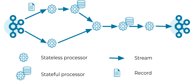
Processors can be stateless or stateful. Stateless processors process records independently of any other data. For example, a processor that implements a map operation (such as masking all but the last four digits of a credit card number) transforms a record into another record without querying any other data. Stateful processors query and maintain a state during the processing of records. For example, an aggregation operation (such as counting the number of input records received in the past five minutes) needs to retrieve the current aggregated value from the state store, update the current aggregated value with the input record, and finally write the new aggregated value to the state store as well as forward the new aggregated value to the downstream processors in the topology. Note that Kafka Streams does not consider processors as stateful if their state is exclusively managed outside of Kafka Streams, that is, when user code within the processor directly calls an external database. While managing state outside of Kafka Streams is possible, we usually recommend managing state inside Kafka Streams to benefit from high performance and processing guarantees.
The topology in the figure above reads records from a Kafka topic and streams the records through a series of stateless and stateful processors. Each processor applies its logic on the input record and forwards an output record to the downstream processors. The last processor in the topology writes its output records to a Kafka topic.
Once a topology is specified, Kafka Streams will execute the topology. Just as a process is an instance of a program that is executed by a computer, a task is an instance of a topology that is executed by Kafka Streams. Kafka Streams creates a task for each partition of the input topic, and each task processes records from its input partition. For example, if the input topic in the topology above has five partitions p0—p4, Kafka Streams will create five tasks t0—t4. Task t0 processes records from partition p0, task t1 processes records from partition p1, and so on. To parallelize the processing, Kafka Streams distributes the five tasks, t0—t4, over all Kafka Streams clients belonging to the same application via the Kafka rebalance protocol.
State store basics
A stateful processor may use one or more state stores. Each task that contains a stateful processor has exclusive access to the state stores in the processor. That means a topology with two state stores and five input partitions will lead to five tasks, and each task will own two state stores resulting in 10 state stores in total for your Kafka Streams application.
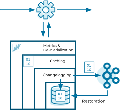
Now that we know how Kafka Streams instantiates state stores, let’s have a look into the internals of them. State stores in Kafka Streams are layered in four ways:
- The outermost layer collects metrics about the operations on the state store and serializes and deserializes the records that are written to and read from the state store.
- The next layer caches the records. If a record exists in the cache with the same key as a new record, the cache overwrites the existing record with the new record; otherwise, the cache adds a new entry for the new record. The cache is the primary serving area for lookups. If a lookup can’t find a record with a given key in the cache, it is forwarded to the next layer. If this lookup returns an entry, the entry is added to the cache. If the cache exceeds its configured size during a write, the cache evicts the records that have been least recently used and sends new and overwritten records downstream. The caching layer decreases downstream traffic because no updates are sent downstream unless the cache evicts records or is flushed. The cache’s size is configurable. If it is set to zero, the cache is disabled.
- The changelogging layer sends each record updated in the state store to a topic in Kafka—the state’s changelog topic. The changelog topic is a compacted topic that replicates the data in the local state. Changelogging is needed for fault tolerance, as we will explain below.
- The innermost layer updates and reads the local state store.
Let’s assume a Kafka Streams application consists of three Kafka Streams clients. While the application executes, one of the Kafka Streams clients crashes. The tasks that the crashed client hosted are redistributed among the two remaining clients. The local states of the crashed client need to be restored on the remaining clients before they can resume processing. However, the remaining clients can’t directly access the local state of the crashed client. Luckily, the changelogging layer sent records to the changelog topic to enable the running clients to restore the local state. This restoration mechanism based on the changelog topic is applied whenever a Kafka Streams client needs to update a local state or needs to create a local state from scratch. In other words, the state’s changelog topic is the single source of truth of a state whereas a state store is a local disposable replica of a partition of the state’s changelog topic that allows you to update and query the state with low latency.
The restoration of a state store is byte based. During restoration, Kafka Streams writes the records from the changelog topic to the local state store without deserializing them. That means the records bypass all layers above the innermost layer during restoration.
The innermost layer of a state store can be any built-in or user-defined state store that implements the state store interface exposed by Kafka Streams. The default state store used in Kafka Streams is RocksDB. Kafka Streams developers initially chose RocksDB because they wanted a write-optimized store. Since RocksDB is the default state store, Kafka Streams provides the means to configure and monitor RocksDB state stores used in a Kafka Streams application.
To configure RocksDB, we need to implement the interface RocksDBConfigSetter and pass the class to the Kafka Streams configuration rocksdb.config.setter. An example for a RocksDB configuration is shown below, where the compaction style of RocksDB is set to level compaction instead of universal compaction that is used by default in Kafka Streams.
public static class MyRocksDBConfig implements RocksDBConfigSetter {
  @Override
  public void setConfig(final String storeName,
                        final Options options,
                        final Map<String, Object> configs) {
    options.setCompactionStyle(CompactionStyle.LEVEL);
  }

  @Override
  public void close(final String storeName, final Options options) {}
}
Besides configuring RocksDB, Kafka Streams also exposes RocksDB-specific metrics to monitor the RocksDB state stores used in a Kafka Streams application. KIP-471 and KIP-607 introduced RocksDB-specific metrics. The former leverages the statistics that are collected by RocksDB and the latter the properties that are exposed by RocksDB. These metrics provide invaluable support for diagnosing and resolving possible issues with RocksDB state stores when operating a Kafka Streams application.
Now that we know the basics of Kafka Streams state stores, we’ll learn how RocksDB works internally and how we can tune it.
Introduction to RocksDB
As you read earlier, the default state store in Kafka Streams is RocksDB. RocksDB is an embeddable key-value persistent store. It is a C++ and Java library that you can embed into your applications. RocksDB is natively designed to give high-end performance for fast storage and server workloads. For example, you can configure RocksDB to provide extremely low query latency on terabytes of data.
Unlike other databases, RocksDB is not a distributed system. It is not highly available and does not have a failover scheme. That doesn’t mean you lose your state store data when you store it in RocksDB using Kafka Streams, because it’s Kafka Streams that makes RocksDB fault tolerant by replicating the state store data to a Kafka topic.
RocksDB is a storage engine library that implements a key-value interface where keys and values are arbitrary bytes. All data is organized in sorted order by the key. RocksDB offers these following operations: Get(key), NewIterator(), Put(key, val), Merge(key, val), Delete(key), and SingleDelete(key). Out of these operations, Kafka Streams specifically calls Get(key), NewIterator(), Put(key, val), and Delete(key).
The operations can be organized into these common categories:
- Updates: You can update keys via the Put and Delete API. Put inserts a single key-value into the database, and Delete removes a single key-value from the database.
- Reads: You can read data via the Get and NewIterator APIs. Get allows an application to fetch a single key-value from the database. An Iterator enables an application to do a RangeScan on the database. The Iterator API can seek to a specified key. Then, the application can start scanning one key at a time from that point, and the keys are returned in sorted order.
- Merges: You can tell RocksDB how to do incremental updates on existing data by avoiding reads. Most databases store data in a disc or a solid-state drive (SSD). An SSD can support a finite amount of I/Os per second. Let’s say you want to do 1 million updates. You will need to perform 1 million reads and 1 million writes—or in other words, 2 million input/output operations per second (IOPS). With the merge operator, you can avoid reads, thus needing only 1 million IOPS. In short, the merge operator in RocksDB helps save half of your disc usage. You can read more about the merge operator on GitHub.
RocksDB architecture overview
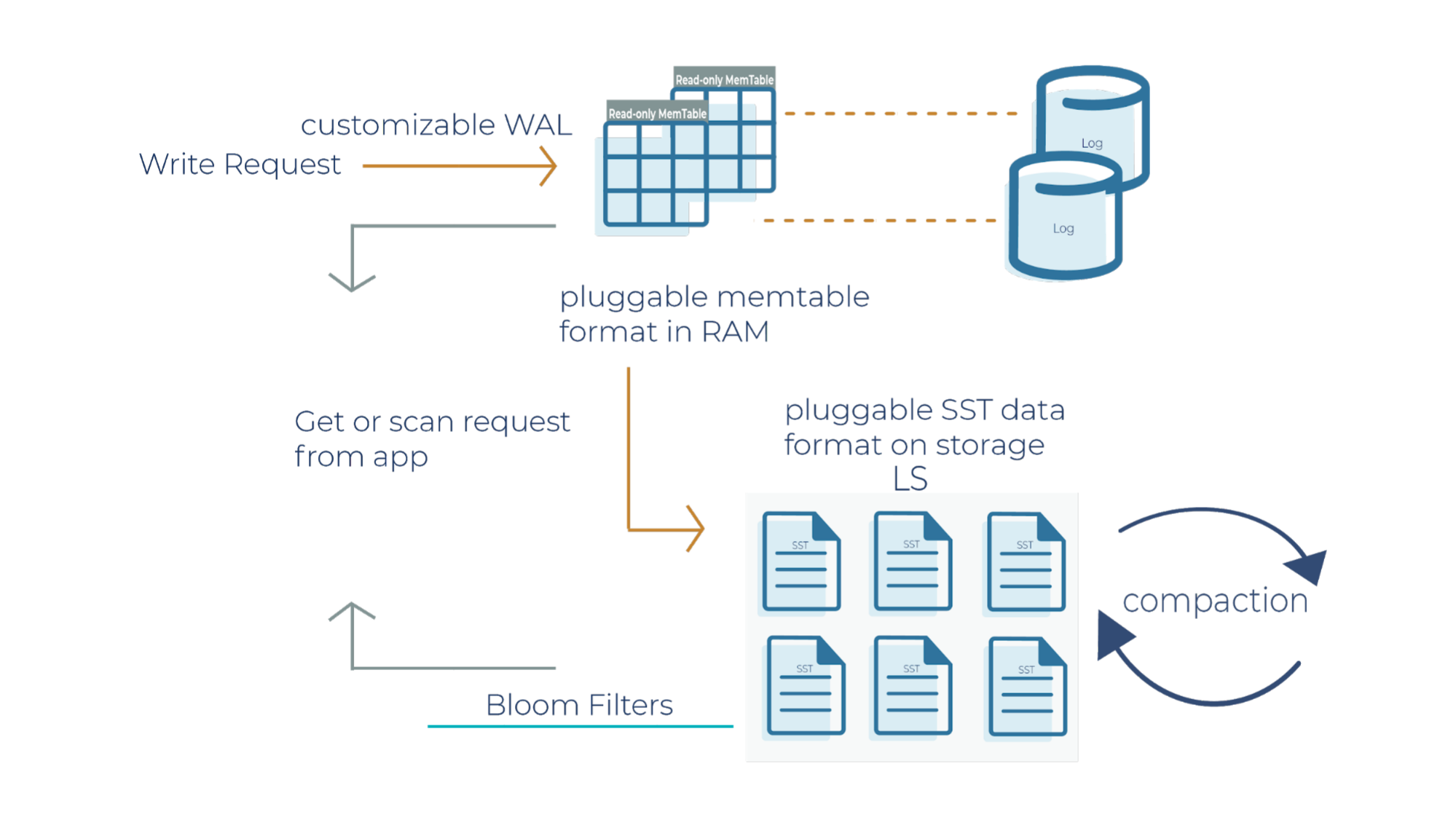
RocksDB uses the log-structured merge architecture to handle high read and write rates on data. In order to debug production applications when you’re running it in a Kafka Streams environment, it helps to understand the architecture of how reads and writes occur. Let’s deep dive into the RocksDB write path.
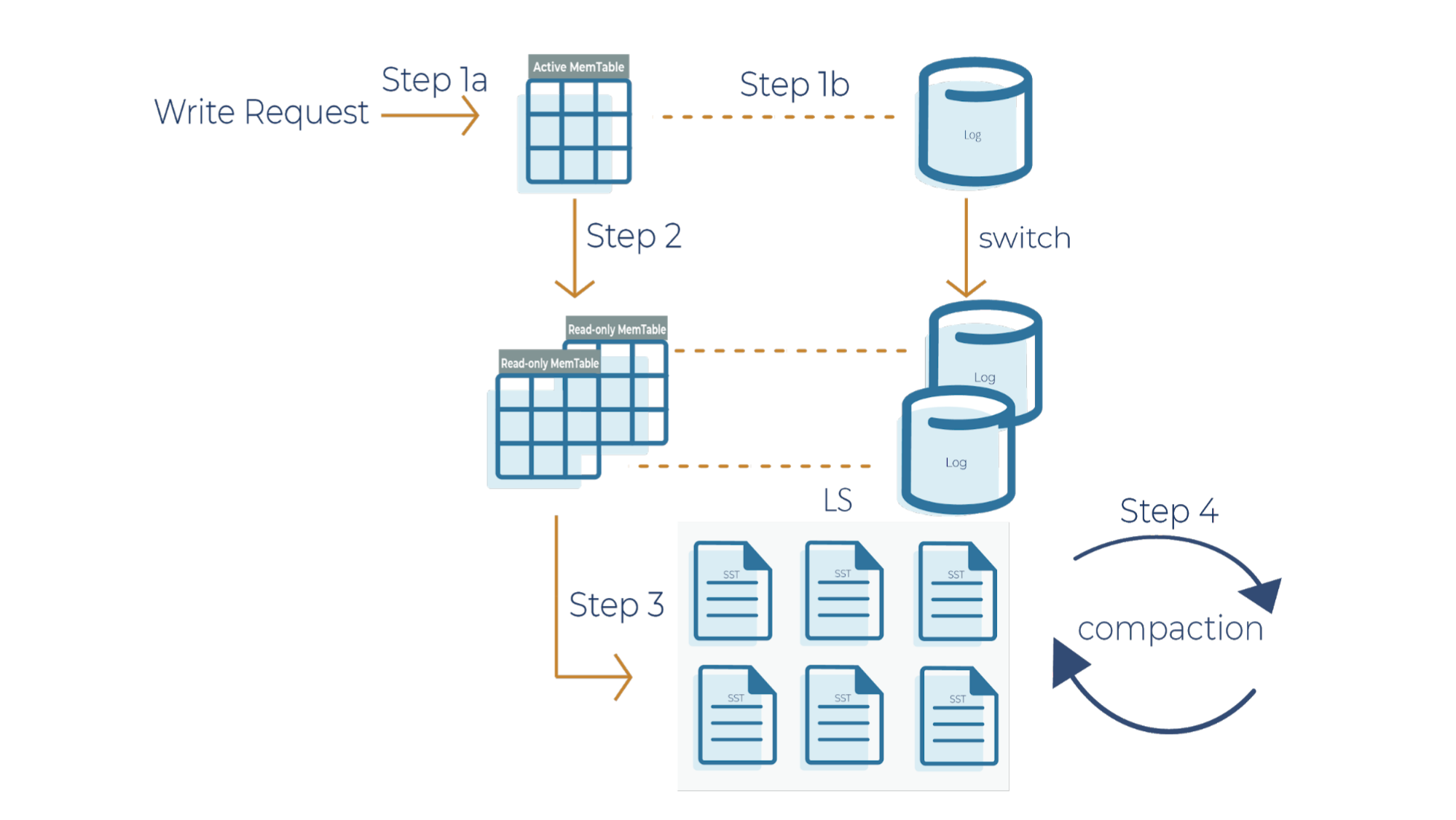
As a side note for the description below, when a write request comes in, it can go to the transaction log and memtable (step 1a and 1b), or it can just go to the memtable only (step 1a). In RocksDB, a transaction log is stored as a log file in storage. You will typically want to use a transaction log if you care about data loss when a database crashes unexpectedly.
A memtable is an in-memory structure where data is buffered. In RocksDB, the default implementation of the memtable is a skip list. However, RocksDB supports a pluggable API that allows an application to provide its own implementation of a memtable. When a memtable fills up, it is flushed to a static sorted table (SST) file on storage.
Step 1a
When there is a write request, it writes to an active memtable, also called a write buffer.
Step 1b
A write request can also directly write to a transaction log. Periodically, the transaction log gets truncated when the SST files persist the data. It’s important to note that in Kafka Streams, the changelog topics replicate the local state stores in Kafka, and hence they behave like transaction logs. As a result, Kafka Streams is configured not to use the RocksDB transaction log.
Step 2
When the memtable is full, it becomes a read-only memtable. From there, new writes continue to accumulate in a new memtable.
Step 3
As new writes accumulate in the new memtable, the read-only memtables are flushed into SST files on the storage system. The data in a SST file is lexicographically sorted to facilitate easy key lookups and sequential scans.
SST files are organized in levels (L0, L1, and so on). Each level has an arbitrary number of SST files. Each SST file has metadata that describes the key range. When you are looking up a particular key, RocksDB checks the metadata to see if a key may exist in a particular file. If it does, it’ll read the file. If it doesn’t, it’ll check the next level. To avoid checking unnecessary files, Bloom filters are used. A Bloom filter is a data structure used to test whether an element is a member of a set. There are Bloom bits (a bit array) that RocksDB keeps for every memtable, and there are also Bloom bits that are stored in every SST file. RocksDB checks Bloom bits first to see if a key may exist in a particular memtable or in a particular SST file. If there is no Bloom match, then we can skip reading the file contents. This is how RocksDB saves on random reads on SST files.
Step 4
This is where periodic compaction occurs. Compaction is a process that lets you maintain the database in reasonable shape and size so that RocksDB performance is maintained. Later on, we’ll cover compaction in more detail.
Now that we have a high-level overview of how Bloom filters function in reducing the number of random reads in SST files, let’s deep dive into the RocksDB read path: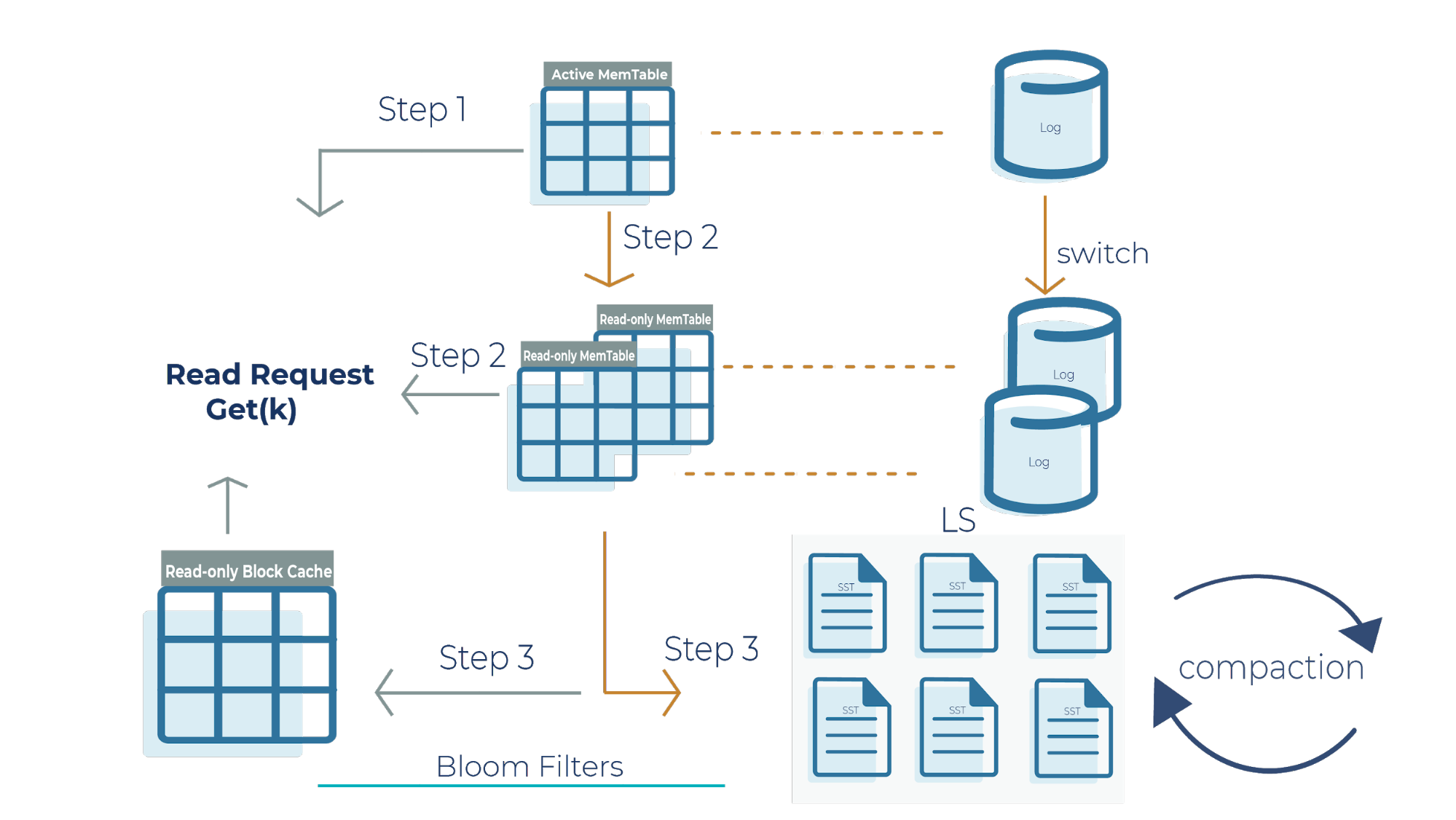
Step 1
When we get a read request, the request looks at the active memtable to see if the key is there because a recent write request may have stored the key there. If we find the key in the active memtable, we don’t need to look at the read-only memtable (step 2) or the SST files (step 3).
Step 2
If the key is not in the active memtable, the request checks the read-only memtable from newest to oldest. It’s important to note that all memtables may have overlapping keys because they contain the most recent datasets that your application writes. If we find the result here, we return it, and we don’t need to look at the SST files (step 3).
Step 3
If we do not find the key in any of the memtables, then the read request checks all the SST files on disk using Bloom filters and returns the value.
Another critical component to highlight in this architecture is the read-only block cache that Kafka Streams uses. It is an in-memory buffer that caches frequently requested keys. It’s important to emphasize that memtables are only used for writes, while the block cache is only used for reads. The memtable and read-only block cache are the two pieces of memory that RocksDB uses to make your database efficient and performant for scaling.
We went into detail with RocksDB’s architecture and how writes and reads operate in RocksDB. One thing we didn’t mention is that RocksDB is highly configurable. Let’s highlight a few main configuration options of RocksDB.
- You can configure the transaction log to be enabled or disabled. Kafka Streams doesn’t use the transaction log in RocksDB because the mentioned changelog topics on the Kafka brokers themselves behave as transaction logs.
- The memtable is a skip list by default. You can configure the memtable to be a vector memtable instead if you want to load data in bulk.
- Another component that you can configure in RocksDB is compaction. We haven’t covered compaction in detail, and we will dive into it in the next section.
Compaction styles in RocksDB
The log structured merge architecture is an append-only data structure. For example, if you delete a key, the deletion is marked and recorded but the key is not immediately removed. Similarly, updates to a key are appended, but the previous value of the key is not updated in place. In order to keep the database size under control, we have to remove all the deleted keys and corresponding delete operations as well as the updated key-value pairs. Compaction is a process of combining a set of SST files and generating new SST files with overwritten keys and deleted keys purged from the output files. Compaction is crucial for securing high performance in RocksDB. There are two basic types of compaction that have different characteristics and are used for different workloads: level compaction and universal compaction.
Level compaction
In level compaction, there are multiple levels (L1-Ln), where an arbitrary number of SST files exist in each level (the green boxes below). L0 is a unique level that contains files just flushed from the memtable: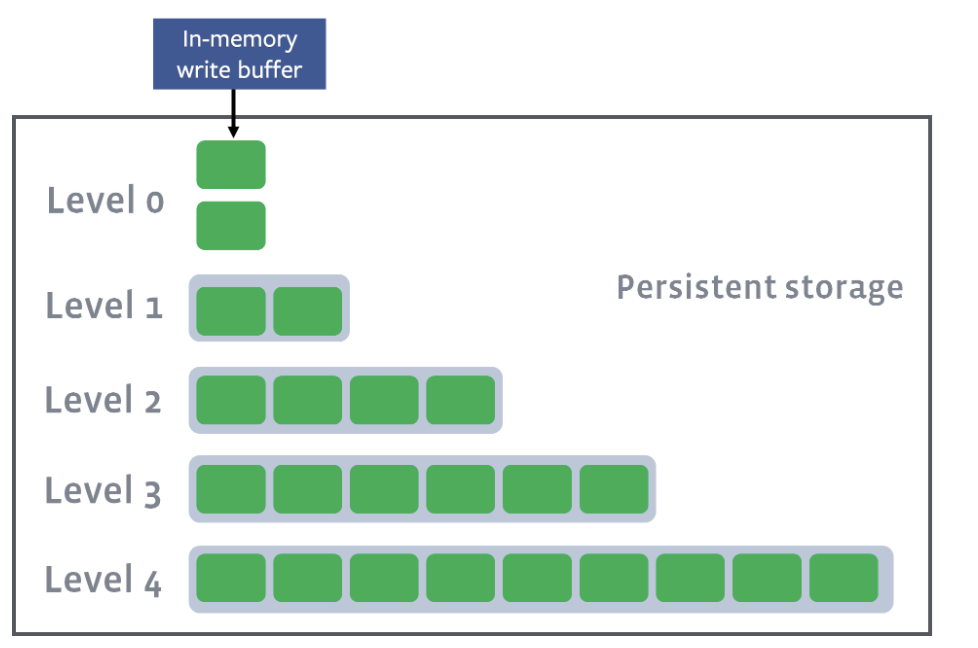
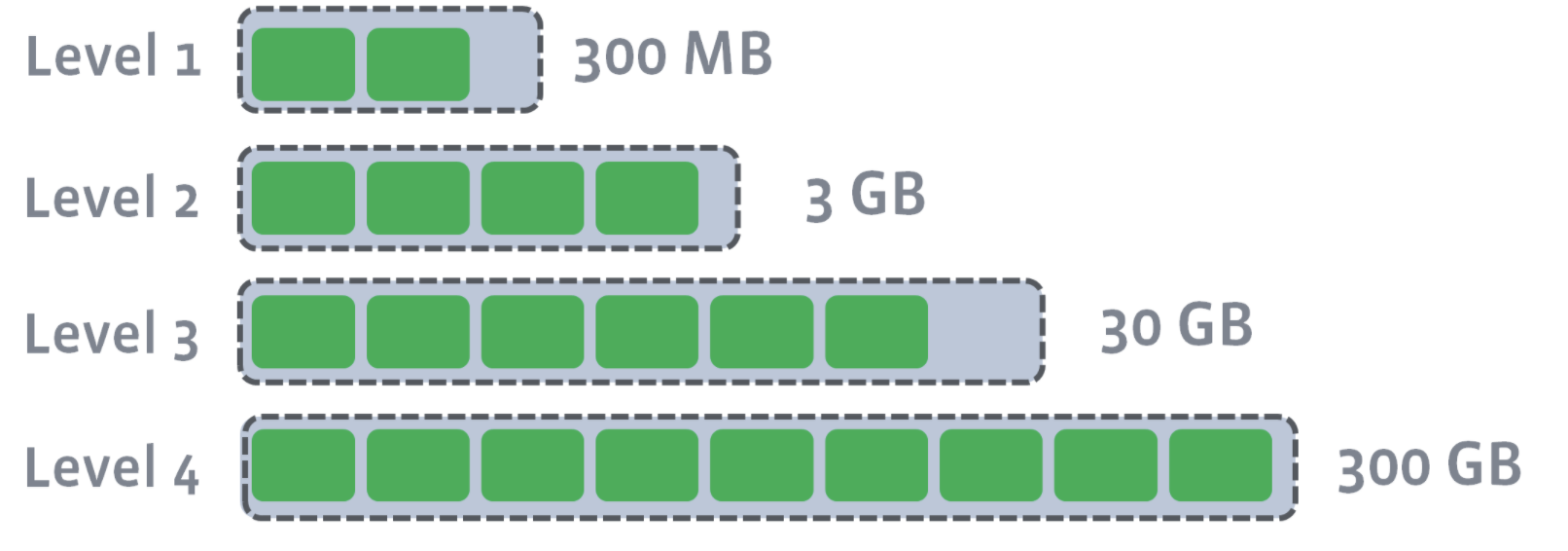
L1–Ln have target sizes. Compaction’s goal is to ensure that L1–Ln is under the target size. Usually, as you move down the level, the target size exponentially increases:
After L0 is compacted with L1, L1’s target size is breached:
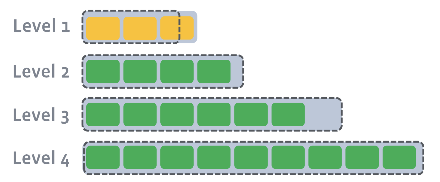
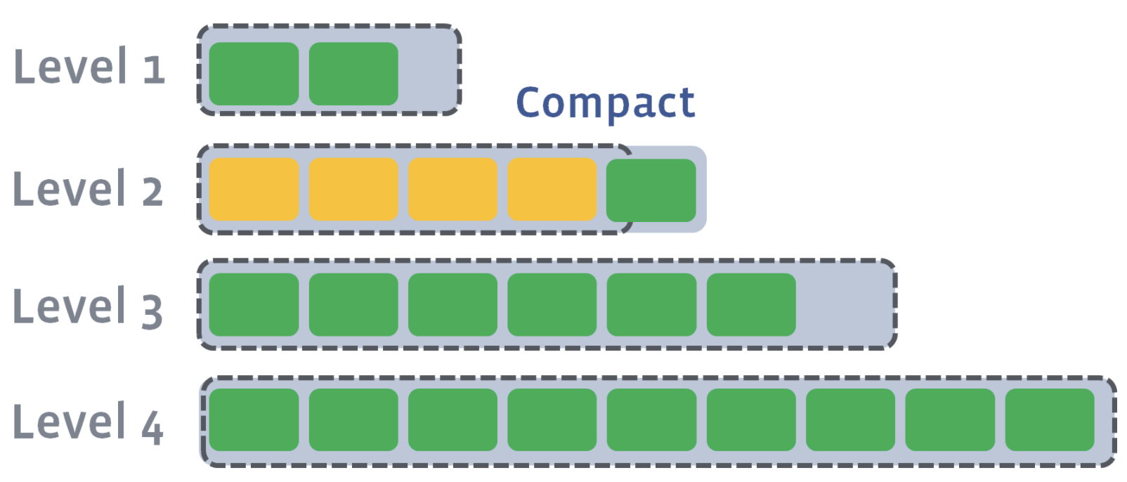
Now, we need to compact L1 with L2. Let’s say that the second SST file on L1 has a newer version of a key where a=4. Let’s also say that the first, second, and third SST file on Level 2 have an older version of a key where a=3, a=2, and a=1. During level compaction, the second SST file on L1 and the first, second, and third SST file on L2 will be merged:
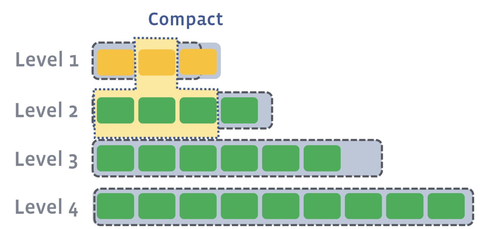
As a result of compaction, four new SST files will be created on L2. One of the SST files will have an updated version of the key, a=4. All other keys in each of the SST files will remain the same. The older versions of the a key will be discarded:
Since L2 has also exceeded its size after compaction, L2 will be compacted into L3. Compaction proceeds from one level to the next until either the target level does not exceed its size or a new target level is created.
Universal compaction
In universal compaction, all SST files are organized in chronological order according to the time that the data was written to the SST files. All data written within a specific time range is stored in an individual SST file or in a “level” in key-range-partitioned SST files. One level stores data written during one time range. Each level is a sorted range of SST files.
For example, we have five sorted runs here: the three files from L0, L4, and L5. L5 is the oldest sorted run, while File0_0 is the newest sorted run.
Level 0: File0_0, File0_1, File0_2
Level 1: (empty)
Level 2: (empty)
Level 3: (empty)
Level 4: File4_0, File4_1, File4_2, File4_3
Level 5: File5_0, File5_1, File5_2, File5_3, File5_4, File5_5
Compaction is triggered in four different ways. For example, one of the ways that compaction can get triggered is if the file is older than the condition set here: options.periodic_compaction_seconds. If the condition is met, then RocksDB proceeds to pick sorted runs for compaction.
Compaction occurs among two or more sorted runs of adjacent time ranges. Compaction merges all sorted runs in one level to create a new sorted run in the next level. Compaction outputs are placed in the highest possible level, where older data is located. Timestamps are stored in the level’s metadata.
If we compact File0_1, File0_2 and L4, the output sorted run will be placed in L4:
Level 0: File0_0,
Level 1: (empty)
Level 2: (empty)
Level 3: (empty)
Level 4: File4_0’, File4_1’, File4_2’, File4_3’
Level 5: File5_0, File5_1, File5_2, File5_3, File5_4, File5_5
Here, L4’s metadata will update to contain the earliest timestamp from File0_1 to the oldest timestamp on File 4_3. New SST files are created from the compaction, specifically File4_0, and older files are discarded. In contrast to level compaction, the size of the level is irrelevant—what matters is the time range of the data in the SST files. For example, all files on L4 are a day old.
Level compaction vs. universal compaction
Level compaction minimizes space amplification, using less disk space compared with universal compaction. However, level compaction does not support as high of write rates as universal compaction. On the other hand, with universal compaction, the disk space can grow up to twice the size of the data in the store.
Kafka Streams uses universal compaction because it supports high write rates. In universal compaction, let’s say we have five SST files with a total size x. When we compact from one level to another, we write no more than the size of the input files, so the write amplification of the compaction job is 1x. In leveled compaction, a set of files of size x in L1 gets compacted with files in L2 that are usually 10 times bigger, so the write amplification of a compaction job would be 11x.
It’s important to note that compaction is multithreaded, which means that different parts of the database could be compacted at the same time by multiple threads. You can configure the number of compaction threads in the system to avoid write stalls (described later on).
How to Tune RocksDB to resolve potential operational issues
In what follows, we’ll describe some operational issues that you may encounter and ways to resolve them.
High memory usage
When your Kafka Streams application has an unexpectedly high memory usage, the RocksDB state stores might be the cause. The symptoms you might experience are:
- Your Kafka Streams application becomes slow or even crashes with out-of-memory errors
- Your operating system shows high memory usage
- These RocksDB-specific metrics exposed by Kafka Streams (introduced with KIP-607 and available in Apache Kafka 2.7 and above) show high values:
- size-all-mem-tables
- block-cache-usage
- block-cache-pinned-usage
- estimate-table-readers-mem
To cope with the high memory usage, you can take the following actions.
Investigate the memtable
The high memory usage can come from the memtables. You’ll have to look at the memtable size and how many memtables you have configured in Kafka Streams. The corresponding options that you can tune in your RocksDBConfigSetter implementation are:
- options.setMaxWriteBufferNumber();
- options.setWriteBufferSize();
Investigate the block cache
For every RocksDB state store in a Kafka Streams application, you have a different block cache. However, you can configure a global block cache. You can share the block cache across all RocksDB state stores that run in one single Kafka Streams client as described in the BoundedMemoryRocksDBConfig in the Kafka Streams documentation. You can even limit the memory used by the shared block cache and memtables of the RocksDB state stores in the same Kafka Streams client by counting the memory used by the memtables against the shared block cache.
Check out RocksDB known bugs
Kafka Streams uses the RocksDB Java API. Certain bugs are memory related that the community is fixing. You can find the known bugs and community information on GitHub.
High disk usage
Similar to high memory usage, you might also experience high disk usage due to RocksDB state stores in your Kafka Streams application. The symptoms you might experience are:
- Application crashes with I/O errors
- Operating system shows high disk usage for the state directories used by RocksDB
- total-sst-files-size (introduced with KIP-607 and available in Apache Kafka 2.7 and above) shows high values.
To cope with the high disk usage, you can take the following actions:
Use level compaction
Kafka Streams uses universal compaction by default for its state stores. However, level compaction has lower space amplification than universal compaction at the cost of lower write rates. The corresponding option that you can tune in your RocksDBConfigSetter implementation is options.setCompactionStyle(CompactionStyle.LEVEL).
Provision more disk space
For universal compaction, some users use a lot of disk space because of the trade-off of space amplification vs. the ability to support a very high write rate. Also, you may experience temporary disk usage spikes. As a rule of thumb, we recommend provisioning more disk space to ensure that you can continue to operate your system without getting errors.
High disk I/O and write stalls
Besides high disk and high memory usage, you might also experience high disk I/O and write stalls. The symptoms you might experience are:
- Operating system shows high disk I/O
- Processing latency of the application increases
- Kafka Streams client gets kicked out of the consumer group
- The following RocksDB-specific metrics exposed by Kafka Streams show high values:
- memtable-bytes-flushed-[rate | total]
- bytes-[read | written]-compaction-rate
- metric write-stall-duration-[avg | total]
- The following RocksDB-specific metrics exposed by Kafka Streams show low values:
- memtable-hit-ratio
- block-cache-[data | index | filter]-hit-ratio
To cope with the high I/O and write stalls, you can take the following actions:
Look at the disk I/O utilization
When you first encounter write stalls, check to see if the hardware is the bottleneck. For example, are you doing too many writes? For this, you can look at I/O utilization.
Check the number of background compaction threads
By default, Kafka Streams configures RocksDB to use as many background compaction threads as the number of available processors, but it configures two background compaction threads if only one processor is available. If you are getting write stalls, manually verify the compaction threads utilization. You can increase the number of background compaction threads in your RocksDBConfigSetter implementation by using options.setIncreaseParallelism().
Increase the number and size of memtables and block cache
All data held in the memtables or block caches do not need to be read from disk when they are looked up; this decreases I/O. You can keep more data in memtables and block caches if you increase their sizes. However, be careful not to run out of memory.
Increase max.poll.interval.ms
The configuration max.poll.interval.ms is the maximum delay between invocations of poll() when using consumer group management (default: five minutes). Once a consumer within a Kafka Streams client exceeds this delay, the consumer is kicked out of the consumer group, leading to recurring rebalances and increased processing lag. If writes to RocksDB stall, the time interval between the invocations of poll() may exceed max.poll.interval.ms. To avoid this, you can increase max.poll.interval.ms in your Kafka Streams application.
Too many open files
By default, Kafka Streams configures RocksDB state stores to not limit the number of open files (i.e., max_open_files = -1). This means that the database opens all the SST files and keeps a file pointer to each one of them. This is great for performance, but you might run out of file descriptors and experience the following symptoms:
- Application crashes with I/O errors
- Kafka Streams metric number-open-files shows high values
To get rid of this issue, you can take the following actions:
Increase the operating system limit
You can increase the operating system limit to a large number and keep the option max_open_files at -1.
Set a limit for open files in RocksDB
You can set RocksDB’s option max_open_files to a number that is less than the limit imposed by the operating system to avoid running out of file descriptors. You can tune the RocksDBConfigSetter implementation via options.setMaxOpenFiles().
Decrease the number of open files
You can decrease the number of open files by setting RockDB’s option target_file_size_base to a larger value, increasing the SST files’ size. For example, the default size of SST files is 64 MB. You could set the option to 128 MB and tune the RocksDBConfigSetter implementation via options.setTargetFileSizeBase().
Summary
Kafka Streams uses RocksDB to maintain local state on a computing node. This blog post went in depth on Kafka Streams state stores and RocksDB architecture, explaining the different ways that you can tune RocksDB to resolve potential operational issues that may arise with Kafka Streams. To learn more about performance tuning RocksDB for Kafka Streams state stores, check out our Kafka Summit session where we delve into this in more detail.
Did you like this blog post? Share it now
Subscribe to the Confluent blog


Why ELT Can't Keep Up in the Era of High-Scale Data Engineering
Batch ELT pipelines create duplication, cost spikes, and governance gaps as data scales. Here’s why enterprises are rethinking legacy integration models.


How to Protect PII in Apache Kafka® With Schema Registry and Data Contracts
Protect sensitive data with Data Contracts using Confluent Schema Registry.