[Webinar] Master Apache Kafka Fundamentals with Confluent | Register Now
Create a Data Analysis Pipeline with Apache Kafka and RStudio
In Data Science projects, we distinguish between descriptive analytics and statistical models running in production. Overall, these can be seen as one process. You start with analyzing historical data to gain insights, find correlations, and finally develop and optimize your model. Then you transfer it and use it in your running system. A key point for every data scientist is not just the mathematical skills themselves, but also how to get the data into your analytics program.
In this blog post, we focus exactly on this crucial step: retrieving the data. In a second article, we’ll talk about running your model on real-time data.
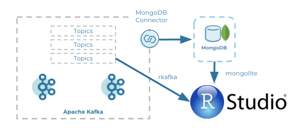
Python, with its Jupyter Notebooks, is commonly used for descriptive analytics. However, the statistical software R also provides deep statistical libraries, and it is my personal first choice when analyzing data. In this tutorial, I’ll explain two ways to create data pipelines from Apache Kafka® into RStudio.
In one method, we use MongoDB as a layer in between, and then we use the R package mongolite to request the data. Using the other method, we consume the data directly using the rkafka package. We also highlight the advantages and drawbacks of each approach (with MongoDB and without MongoDB).
On GitHub, you can find all code for the Mongo DB and rkafka pipelines.
Setup
Prerequisites: docker, docker-compose, (MongoDB Compass)
For configurations, we focus on simplicity so that our settings here can be used as a baseline for similar projects. For example, the Kafka topic is in JSON value format so that we do not need a schema registry. Our starting position is a simple Kafka producer producing data every two seconds of a truck driving from Hamburg to Munich in Germany. One example event looks like this:
{
“latitude”: 53.56067,
“longitude”: 9.9908,
“speed_kmh”: 105.564,
“timestamp”: “2021-05-23T11:39:00.000Z”
}
With docker-compose up -d, we start all containers:
- Zookeeper
- Kafka Broker (for more information about its configurations, see the documentation)
- KAFKA_AUTO_CREATE_TOPICS_ENABLE: “true” ensures that we do not need to manually create the Kafka topic in which the producer sends its messages
- Kafka Producer
- a Docker image built to execute the fat JAR that continuously produces fake data
For with MongoDB we also start:
-
- Kafka Connect (for more information about its configurations, see the documentation)
- CONNECT_CONNECTOR_CLIENT_CONFIG_OVERRIDE_POLICY: “All” allows us to change the offset from latest to earliest of the MongoDB Connector, since we want to have all historical data
- Note: The MongoDB Sink Connector is not part of the default connectors. Therefore, we download it from Confluent Hub and run it with a Bash command
- MongoDB
- RStudio
- Kafka Connect (for more information about its configurations, see the documentation)
For without MongoDB we also start:
- RStudio
- with the rJava and rkafkajars packages already installed because they are required for rkafka
Kafka Producer
The Kafka Producer is written in Kotlin using Kafka Streams (version 2.7.0) and has the following properties:
KEY_SERIALIZER_CLASS_CONFIG: “org.apache.kafka.common.serialization.StringSerializer”,
VALUE_SERIALIZER_CLASS_CONFIG: “org.apache.kafka.common.serialization.StringSerializer”,
BOOTSTRAP_SERVER_CONFIG: “broker:29092”
We define how to serialize our key and value as well as setting the broker address. Notice that we use the external port of the broker, instead of the internal one. The article Running Kafka in Docker Machine, by Marcelo Hossomi, explains the reason very well—I wish I would have read it before making the same mistakes.
We can verify that data is correctly produced into the Kafka topic truck-topic by running the commands docker-compose exec broker bash and kafka-console-consumer --bootstrap-server broker:9092 --topic truck-topic.
MongoDB Sink Connector
When using the pipeline option with MongoDB, we need to configure a MongoDB Sink Connector and start it. Our connector has the following configurations:
{
 "name": "TestData",
 "config": {
   "name": "TestData",
   "connector.class": "com.mongodb.kafka.connect.MongoSinkConnector",
   "key.converter": "org.apache.kafka.connect.storage.StringConverter",
   "key.converter.schemas.enable": "false",
   "value.converter": "org.apache.kafka.connect.json.JsonConverter",
   "value.converter.schemas.enable": "false",
   "topics": "truck-topic",
   "consumer.override.auto.offset.reset": "earliest",
   "connection.uri": "mongodb://user:password@mongo:27017/admin",
   "database": "TruckData",
   "collection": "truck_1"
 }
}
This takes the truck-topic from the beginning and stores it in the MongoDB database TruckData in the truck_1 collection. When working with the Avro format, you can find the additional configurations in the MongoDB documentation. We then start the connector via the command curl -X POST -H "Content-Type: application/json" --data @MongoDBConnector.json http://localhost:8083/connectors | jq, and verify that the connector is running using the command curl localhost:8083/connectors/TestData/status | jq.
MongoDB Compass
Now, we start MongoDB Compass and create a new connection with username: user, password: password, authentication database: admin, or directly using URI: mongodb://user:password@localhost:27017/admin. We see the data in the TruckData database in the truck_1 collection.
Moreover, we can apply aggregations and export those for other programs. Here, we filter the data to have a timestamp greater than or equal to 2021-05-23. Unfortunately, it is not possible to export the query for R, but we’ll see later on how we can adapt it so that it is executable.
RStudio
To start the descriptive analysis, we now need to request the data, which is stored in our Kafka topic truck-topic (as well as in MongoDB). We can start RStudio on localhost:8787 with user: user and password: password. Under the /home directory, we find our corresponding R files.
mongolite
We create a connection to MongoDB and then request all of the data with connection$find(). We also can use the aggregation pipeline defined in MongoDB Compass. To do so, we replace all ‘ (single quotes) with ‘’ (double quotes) and then paste the query into connection$aggregate(‘ ’).
rkafka
We want to be able to read the data multiple times, so we first create a simple Consumer with some configurations:
kafkaServerURL: “broker”,
kafkaServerPort: “9092”,
connectionTimeOut: “10000”,
kafkaProducerBufferSize: “100000”,
clientId: “truck-topic”
We then iterate over the offset from partition 0, consuming the data from the beginning and creating a data frame out of it. To convert the JSON string, we use the jsonlite package.
Which pipeline should I use?
There are pros and cons for both styles of pipeline. The most straightforward way is to use rkafka and consume the data from the topic itself. By iterating over the offset, we can define how large our data frame maximal will be and specify that we want to consume from the beginning (offset = 0). However, we cannot directly query the data, such as for a specific time interval or the total number of events. Moreover, we created the pipeline locally without configuring any authentication. Reading the package documentation, I could not find how to deal with this issue.
Using MongoDB as a layer in between results in a more complicated setup. We need to start Kafka Connect, add the connector as a plugin, configure it, and start it. However, we can directly see in MongoDB Compass how large the data set is, we can do aggregations on the data using the aggregation pipeline, and we can convert those when requesting the data in RStudio.
In the end, the best approach depends on the circumstances of the project, as well as personal preferences. We now have the data as a data frame in RStudio, and we can start our actual work: analyzing it.
Conclusion
In this tutorial, we implemented two methods of transferring historical data from Apache Kafka into R. In the future, we will take a look at using our defined models on real-time data. If you have problems when executing the tutorial or have any questions, feel free to reach out in the Community Forum or Slack.
Did you like this blog post? Share it now
Subscribe to the Confluent blog


Introducing KIP-848: The Next Generation of the Consumer Rebalance Protocol
Big news! KIP-848, the next-gen Consumer Rebalance Protocol, is now available in Confluent Cloud! This is a major upgrade for your Kafka clusters, offering faster rebalances and improved stability. Our new blog post dives deep into how KIP-848 functions, making it easy to understand the benefits.
How to Query Apache Kafka® Topics With Natural Language
The users who need access to data stored in Apache Kafka® topics aren’t always experts in technologies like Apache Flink® SQL. This blog shows how users can use natural language processing to have their plain-language questions translated into Flink queries with Confluent Cloud.