New in Confluent Cloud: Making Data & Pipelines Accessible for AI-Ready Streaming | Learn More
Learning All About Wi-Fi Data with Apache Kafka and Friends
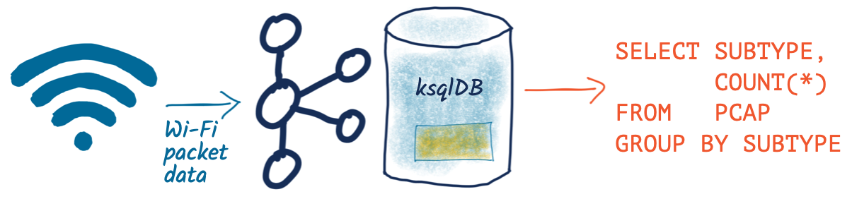
Recently, I’ve been looking at what’s possible with streams of Wi-Fi packet capture (pcap) data. I was prompted after initially setting up my Raspberry Pi to capture pcap data and stream it to Apache Kafka®. Because I was using Confluent Cloud, it was easy enough to chuck the data at the Kafka cluster and not worry about where or how to run it. I set this running a month ago, and with a few blips in between (my Raspberry Pi is not deployed for any nines of availability!), I now have a bunch of raw pcap data that I thought would be interesting to dig into using Kafka and its surrounding ecosystem.
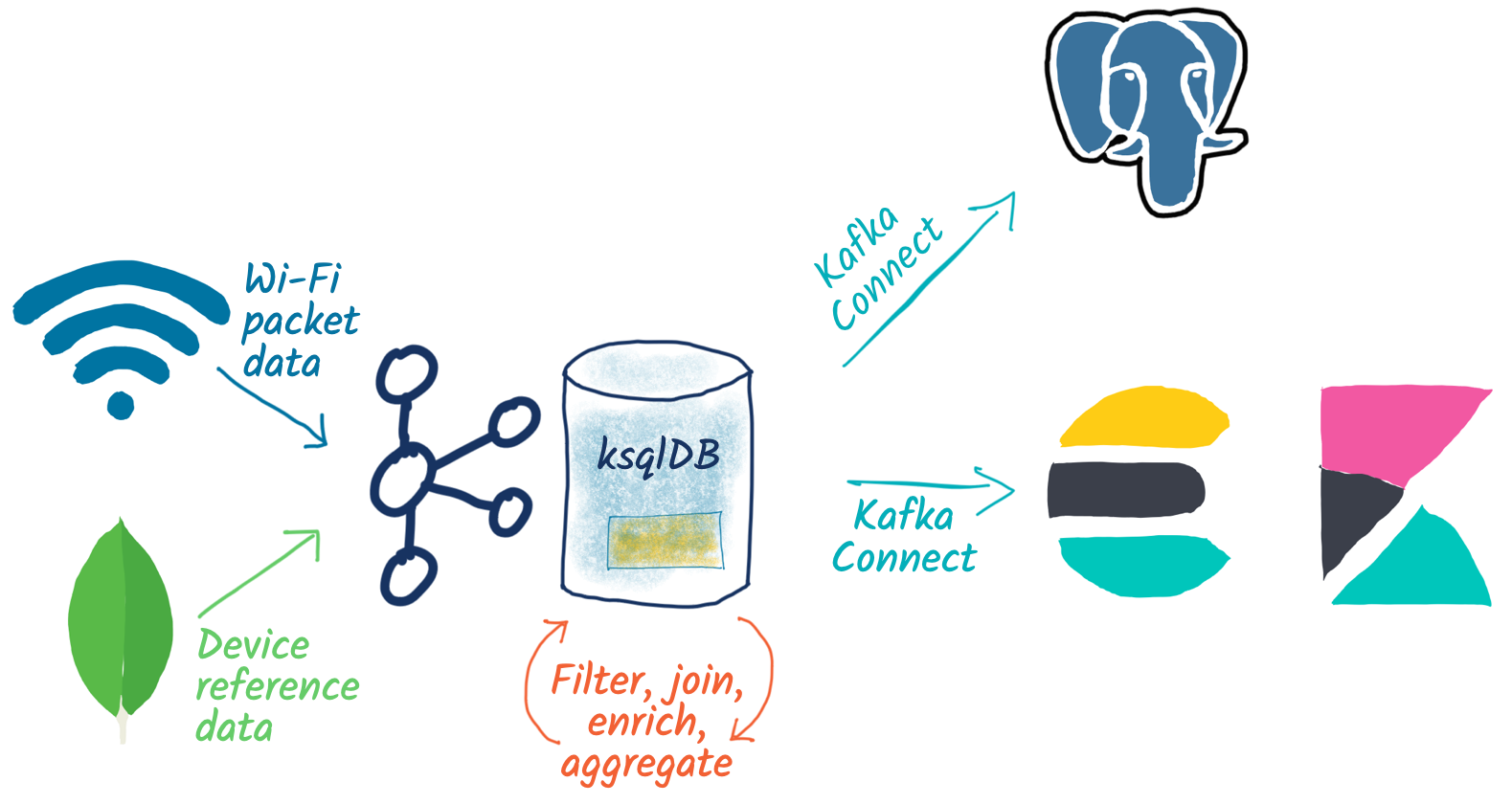
In a nutshell, what I end up with is a pipeline for processing the pcap data, joining it to reference data from an external system, aggregating it, and streaming it to various datastores, including Neo4j and PostgreSQL.
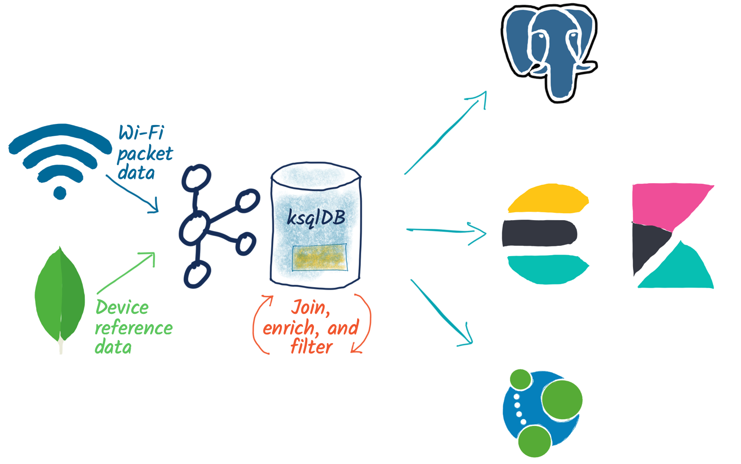
At the heart of the data is wlan pcap data captured from tshark (the command line equivalent of Wireshark). The data is stored in JSON on a partitioned Kafka topic, and a sample message looks like this:
{
  "timestamp": "1584802202655",
  "wlan_fc_type": [ "1" ],
  "wlan_fc_type_subtype": [ "25" ],
  "wlan_radio_channel": [ "1" ],
  "wlan_radio_signal_dbm": [ "-73" ],
  "wlan_radio_duration": [ "32" ],
  "wlan_ra": [ "a4:fc:77:6c:55:0d" ],
  "wlan_ra_resolved": [ "MegaWell_6c:55:0d" ],
  "wlan_ta": [ "48:d3:43:43:cd:d1" ],
  "wlan_ta_resolved": [ "ArrisGro_43:cd:d1" ]
}
These messages come in at a rate of about 100,000 per hour, or c.30 per second. That’s not “big data,” but it’s not insignificant either.
It certainly gives me a bunch of data that’s more than I can grok by just poking around it. I don’t really know what I’m looking for in the data quite yet, I’m just interested in what I’ve scooped up in my virtual net. Let’s take two approaches: one visual and one numeric to see if we can get a better handle on the data.
Understanding the overall dataset visually
First, I wanted a visual glimpse of the data to better understand usage volumes. Kibana has a nice tool as part of its machine learning feature called Data Visualizer. Let’s stream our raw Wi-Fi packet captures into Elasticsearch and check it out.

curl -i -X PUT -H  "Content-Type:application/json" \
    http://localhost:8083/connectors/sink-elastic-pcap-00/config \
    -d '{
        "connector.class": "io.confluent.connect.elasticsearch.ElasticsearchSinkConnector",
        "topics": "pcap",
        "value.converter": "org.apache.kafka.connect.json.JsonConverter",
        "value.converter.schemas.enable": "false",
        "connection.url": "http://elasticsearch:9200",
        "type.name": "_doc",
        "key.ignore": "true",
        "schema.ignore": "true"
    }'
Here, we can see characteristics in the data including:
- Record count per day
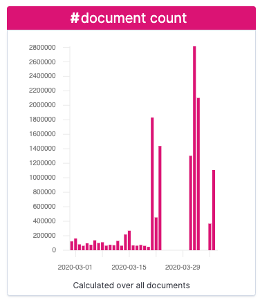
- The distribution of MAC addresses in senders (sa) and receivers (ra)
- Which types of packets are most commonly found (wlan_fc_subtype)
Based on this published table, we can see the most common types of packets are:
- 33% ACK (wlan.fc.type_subtype == 29)
- 20% Request to Send (wlan.fc.type_subtype == 27)
- 13% Probe Request (wlan.fc.type_subtype == 4)
- 11% NULL Data (wlan.fc.type_subtype == 36)
What about getting these numbers from analysing the data directly from the console, without using Elasticsearch?
Understanding the overall dataset numerically
With ksqlDB, you can use SQL queries to inspect, aggregate, and process data. Let’s see it in action with the raw pcap data that we’ve got.
First up, I’m going to declare a schema so that I can query attributes of the data in the topic. The full schema is pretty beefy and since I’m only interested in a couple of fields at this point (the date and the subtype ranges), I’m just going to specify a partial schema at this stage.
CREATE STREAM PCAP_RAW_00 (timestamp            BIGINT,
                           wlan_fc_type_subtype ARRAY<INT>)
    WITH (KAFKA_TOPIC='pcap',
          VALUE_FORMAT='JSON',
          TIMESTAMP='timestamp');
A couple of things to point out:
- Notice that the wlan_fc_type_subtype is written by the source application (tshark) as an array of INT, e.g., "wlan_fc_type": [ "1" ]
- I tell ksqlDB to take the timestamp field from the payload as the timestamp of the message (WITH … TIMESTAMP='timestamp')If I didn’t do this, it would default to the timestamp of the Kafka message held in the message’s metadata, which is not what I want in this case. Since we’re going to analyse the time attributes of the data, it’s important to correctly handle event time vs. ingest time here.
With the stream created, I tell ksqlDB to process the data from the beginning of the topic:
SET 'auto.offset.reset' = 'earliest';
And then query it using SQL:
SELECT wlan_fc_type_subtype[1] AS SUBTYPE,
       COUNT(*) AS PACKET_COUNT,
       TIMESTAMPTOSTRING(MIN(ROWTIME),'yyyy-MM-dd HH:mm:ss','GMT') AS MIN_TS,
       TIMESTAMPTOSTRING(MAX(ROWTIME),'yyyy-MM-dd HH:mm:ss','GMT') AS MAX_TS
FROM   PCAP_RAW_00 WHERE ROWTIME < (UNIX_TIMESTAMP() - 1800000)
GROUP BY wlan_fc_type_subtype[1]
EMIT CHANGES;
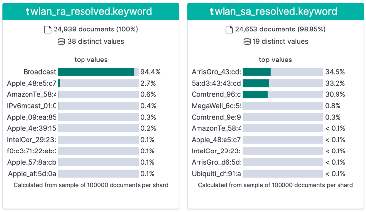
Here, we’re aggregating all messages received up until the last half hour by subtype, but you’ll notice that it’s calculating the numbers from the start of the topic and continually updating as newer messages are processed:
To build on this example, let’s break down the subtype count by day. You’ll notice that instead of writing the aggregate result to the screen, we’re instantiating it as a table within ksqlDB:
SET 'auto.offset.reset' = 'earliest';
CREATE TABLE PCAP_STATS WITH (VALUE_FORMAT='AVRO') AS
SELECT TIMESTAMPTOSTRING(WINDOWSTART,'yyyy-MM-dd','GMT') AS WINDOW_DAY,
       WLAN_FC_TYPE_SUBTYPE[1] AS SUBTYPE,
       COUNT(*) AS PACKET_COUNT,
       TIMESTAMPTOSTRING(MIN(ROWTIME),'HH:mm:ss','GMT') AS EARLIEST_TIME,
       TIMESTAMPTOSTRING(MAX(ROWTIME),'HH:mm:ss','GMT') AS LATEST_TIME
FROM   PCAP_RAW_00
        WINDOW TUMBLING (SIZE 1 DAY)
GROUP BY WLAN_FC_TYPE_SUBTYPE[1]
EMIT CHANGES;
Now there’s an actual materialised view of this data, backed by a persisted Kafka topic:
ksql> SHOW TABLES;

 Table Name | Kafka Topic | Format | Windowed
----------------------------------------------
 PCAP_STATS | PCAP_STATS  | AVRO   | false
----------------------------------------------
We can query this table using either a push query, showing all updates as they arrive:
Or we can query the value directly with a pull query for any of the subtypes:
ksql> SELECT WINDOW_DAY, SUBTYPE, PACKET_COUNT, EARLIEST_TIME, LATEST_TIME
        FROM PCAP_STATS
       WHERE ROWKEY = 4 ;
+-----------+--------+-------------+--------------+------------+
|WINDOW_DAY |SUBTYPE |PACKET_COUNT |EARLIEST_TIME |LATEST_TIME |
+-----------+--------+-------------+--------------+------------+
|2020-02-28 |4       |84           |22:47:06      |23:59:35    |
|2020-02-29 |4       |3934         |00:02:01      |23:58:19    |
|2020-03-01 |4       |1601         |00:00:06      |23:58:07    |
|2020-03-02 |4       |1125         |00:00:12      |23:59:13    |
Query terminated
Since it’s just a Kafka topic, you can persist this aggregate to a database, using the message key to ensure that values update in place. To do this, we’ll use Kafka Connect like we did above for Elasticsearch, but instead of calling the Kafka Connect REST API natively, here we’ll use ksqlDB as the interface for creating the connector:
CREATE SINK CONNECTOR SINK_POSTGRES_PCAP_STATS_00 WITH (
    'connector.class'     = 'io.confluent.connect.jdbc.JdbcSinkConnector',
    'connection.url'      = 'jdbc:postgresql://postgres:5432/',
    'connection.user'     = 'postgres',
    'connection.password' = 'postgres',
    'topics'              = 'PCAP_STATS',
    'key.converter'       = 'org.apache.kafka.connect.storage.StringConverter',
    'auto.create'         = 'true',
    'auto.evolve'         = 'true',
    'insert.mode'         = 'upsert',
    'pk.mode'             = 'record_value',
    'pk.fields'           = 'WINDOW_DAY,SUBTYPE',
    'table.name.format'   = '${topic}'
);
Now as each message arrives in the source Kafka topic, it’s incorporated in the aggregation by ksqlDB, and the resulting change to the aggregate is pushed to Postgres, where each key (which is a composite of the SUBTYPE plus the day) is updated in place:
postgres=# SELECT * FROM "PCAP_STATS" WHERE "SUBTYPE"=4 ORDER BY "WINDOW_DAY" ;
 WINDOW_DAY | SUBTYPE | PACKET_COUNT | EARLIEST_TIME | LATEST_TIME
------------+---------+--------------+---------------+-------------
 2020-02-28 |       4 |           89 | 22:47:25      | 23:55:44
 2020-02-29 |       4 |         4148 | 00:02:01      | 23:58:19
 2020-03-01 |       4 |         1844 | 00:00:24      | 23:56:53
 2020-03-02 |       4 |          847 | 00:00:12      | 23:59:13
…
Analysing relationships in the data with Kibana
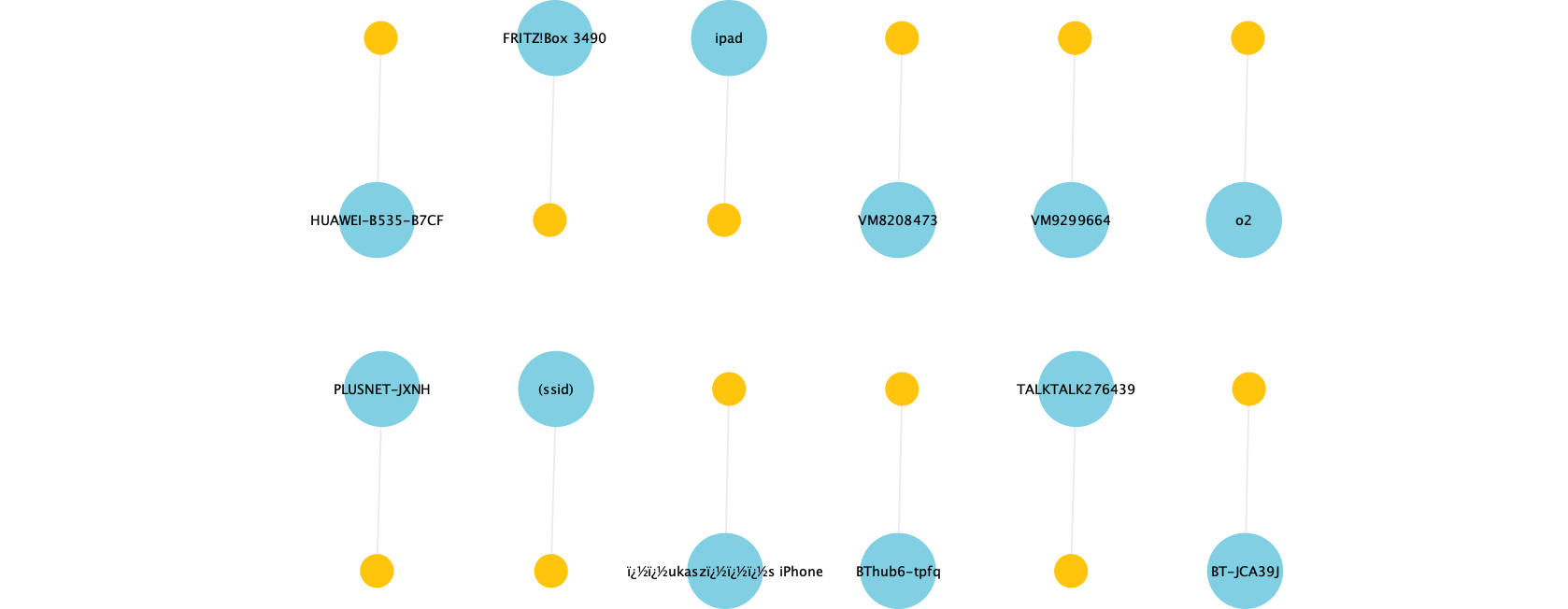
Similar to the Data Visualizer in Kibana, the graph capabilities are also helpful for exploring high-level relationships in the data.
By looking at a few of the key entities, we can observe which devices (yellow circles) scan which access points (light blue circles), as well as how frequently (thickness of connecting lines). We can also see the clustering that occurs between devices and the access points that they scan. This pattern of analysis is evidently a fruitful avenue for investigation, and later in this article, we’ll do some dedicated graph modelling and analysis of the data by streaming the data from Kafka into Neo4j and analysing it there.
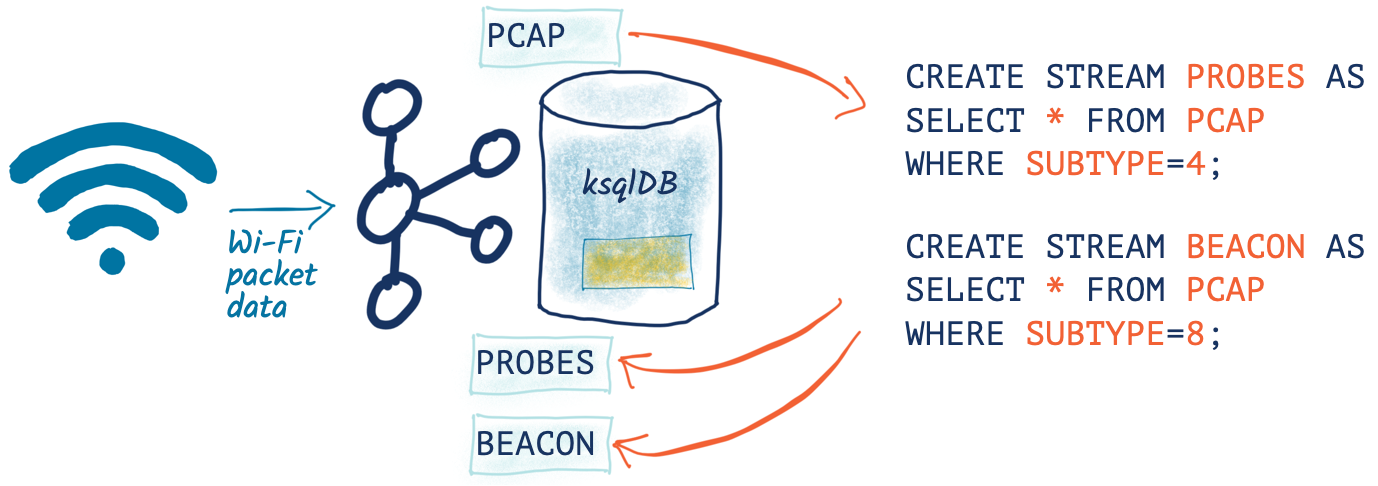
Splitting the pcap data into separate topics
Having identified the types of data within the pcap stream, let’s now use ksqlDB to split the data into separate topics for further analysis. The separate topics will make the analysis easier to target on the correct stream of data and also allow each type of data to have a different schema.
To begin, I’ll declare a schema that covers fields across all types of packet:
CREATE STREAM pcap_raw (timestamp                    BIGINT,
                        wlan_fc_type_subtype         ARRAY<INT>,
                        wlan_radio_channel           ARRAY<INT>,
                        wlan_radio_signal_percentage ARRAY<VARCHAR>,
                        wlan_radio_signal_dbm        ARRAY<DOUBLE>,
                        wlan_radio_duration          ARRAY<INT>,
                        wlan_ra                      ARRAY<VARCHAR>,
                        wlan_ra_resolved             ARRAY<VARCHAR>,
                        wlan_da                      ARRAY<VARCHAR>,
                        wlan_da_resolved             ARRAY<VARCHAR>,
                        wlan_ta                      ARRAY<VARCHAR>,
                        wlan_ta_resolved             ARRAY<VARCHAR>,
                        wlan_sa                      ARRAY<VARCHAR>,
                        wlan_sa_resolved             ARRAY<VARCHAR>,
                        wlan_staa                    ARRAY<VARCHAR>,
                        wlan_staa_resolved           ARRAY<VARCHAR>,
                        wlan_tagged_all              ARRAY<VARCHAR>,
                        wlan_tag_vendor_data         ARRAY<VARCHAR>,
                        wlan_tag_vendor_oui_type     ARRAY<VARCHAR>,
                        wlan_tag_oui                 ARRAY<VARCHAR>,
                        wlan_country_info_code       ARRAY<VARCHAR>,
                        wps_device_name              ARRAY<VARCHAR>,
                        wlan_ssid                    ARRAY<VARCHAR>)
    WITH (KAFKA_TOPIC='pcap',
        VALUE_FORMAT='JSON',
        TIMESTAMP='timestamp');
Now we can pull out records of different types into new streams and take the opportunity to serialise the resulting data to Apache Avro™. Using Avro (or similar serialisation options that include strong support for schemas, like Protobuf) is helpful because we’ve already declared the schema once for the data, and serialising it to Avro means that when we—or anyone else—consumes the data from the topic, the schema is available without having to reenter it. It also provides compatibility checks on the validity of the schema when writing to the topic.
SET 'auto.offset.reset' = 'earliest';
CREATE STREAM PCAP_PROBE  WITH (VALUE_FORMAT='AVRO') AS SELECT * FROM PCAP_RAW WHERE WLAN_FC_TYPE_SUBTYPE[1]=4;
CREATE STREAM PCAP_BEACON WITH (VALUE_FORMAT='AVRO') AS SELECT * FROM PCAP_RAW WHERE WLAN_FC_TYPE_SUBTYPE[1]=8;
CREATE STREAM PCAP_RTS    WITH (VALUE_FORMAT='AVRO') AS SELECT * FROM PCAP_RAW WHERE WLAN_FC_TYPE_SUBTYPE[1]=27;
CREATE STREAM PCAP_CTS    WITH (VALUE_FORMAT='AVRO') AS SELECT * FROM PCAP_RAW WHERE WLAN_FC_TYPE_SUBTYPE[1]=28;
CREATE STREAM PCAP_ACK    WITH (VALUE_FORMAT='AVRO') AS SELECT * FROM PCAP_RAW WHERE WLAN_FC_TYPE_SUBTYPE[1]=29;
CREATE STREAM PCAP_NULL   WITH (VALUE_FORMAT='AVRO') AS SELECT * FROM PCAP_RAW WHERE WLAN_FC_TYPE_SUBTYPE[1]=36;
If we had a partition key strategy that we wanted to apply, we could do this by specifying PARTITION BY—but since we’re still at the early stages of analysis, we’ll leave the key unset for now (which means that messages will be distributed “round robin” evenly across all partitions). We could also opt to drop unused columns from the schema for particular message types by replacing SELECT * with a specific projection of required columns.
This creates and populates new Kafka topics:
ksql> SHOW TOPICS;

 Kafka Topic                            | Partitions | Partition Replicas
--------------------------------------------------------------------------
 PCAP_ACK                               | 12         | 3
 PCAP_BEACON                            | 12         | 3
 PCAP_CTS                               | 12         | 3
 PCAP_NULL                              | 12         | 3
 PCAP_PROBE                             | 12         | 3
 PCAP_RTS                               | 12         | 3
 PCAP_STATS                             | 12         | 3
 …
Analysing Wi-Fi probe requests
Mobile devices send probe requests to see what access points (AP) are available, which provides a good source of data for analysis. I was curious how often my Wi-Fi network is probed by both familiar and unfamiliar devices. Kibana is a great tool here for “slicing and dicing” the data to explore that question. By adding a filter for the subtype, we can easily pick out the fields that have relevant data:
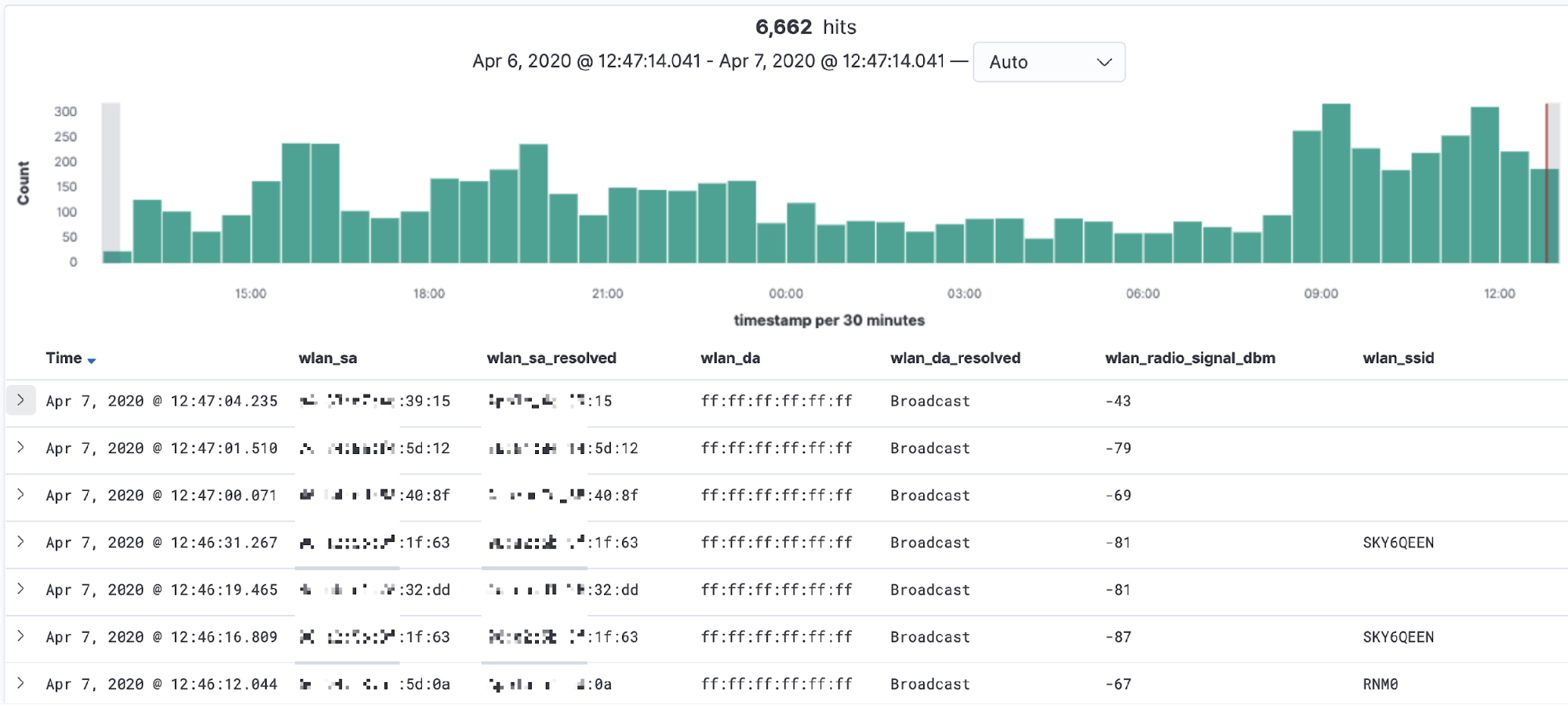
- wlan_sa is the raw source MAC address, whilst wlan_sa_resolved includes, in some cases, the manufacturer’s prefix
- Most requests look for any AP, but some are for a specific wireless network (wlan_ssid)
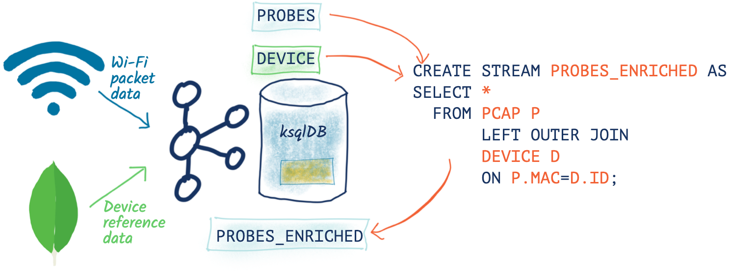
Enriching pcap data with lookups
So in all this “digital exhaust” is a load of devices from within my house, plus others externally. Wouldn’t it be nice to be able to identify them? This is where the real power of ksqlDB comes in, because I can use it to join a stream of events (pcap data) with lookup data from elsewhere.
My Ubiquiti router uses MongoDB to store details of all my household devices that use it across two separate MongoDB collections. Let’s pull that data into Kafka through ksqlDB:
CREATE SOURCE CONNECTOR SOURCE_MONGODB_UNIFI_01 WITH (
    'connector.class' = 'io.debezium.connector.mongodb.MongoDbConnector',
    'mongodb.hosts' = 'rs0/mongodb:27017',
    'mongodb.name' = 'unifi',
    'collection.whitelist' = 'ace.device, ace.user'
);
With this data in Kafka, we can use some data wrangling tricks to build two ksqlDB tables of devices (switches, APs, and routers) and users (i.e., Wi-Fi clients—mobiles, laptops, etc.). To get more background on what this ksqlDB code does and why, check out this article.
-- Model source topics
CREATE STREAM DEVICES_RAW WITH (KAFKA_TOPIC='unifi.ace.device', VALUE_FORMAT='AVRO');
CREATE STREAM USERS_RAW   WITH (KAFKA_TOPIC='unifi.ace.user',   VALUE_FORMAT='AVRO');

-- Extract device data fields from JSON payload
SET 'auto.offset.reset' = 'earliest';
CREATE STREAM ALL_DEVICES WITH (PARTITIONS=12,
                                KAFKA_TOPIC='all_devices_00') AS
        SELECT  'ace.device'                       AS SOURCE,
                EXTRACTJSONFIELD(AFTER ,'$.mac')   AS MAC,
                EXTRACTJSONFIELD(AFTER ,'$.ip')    AS IP,
                EXTRACTJSONFIELD(AFTER ,'$.name')  AS NAME,
                EXTRACTJSONFIELD(AFTER ,'$.model') AS MODEL,
                EXTRACTJSONFIELD(AFTER ,'$.type')  AS TYPE,
                CAST('0' AS BOOLEAN)               AS IS_GUEST
        FROM    DEVICES_RAW
        -- Set the MAC address as a the message key
        PARTITION BY EXTRACTJSONFIELD(AFTER ,'$.mac')
        EMIT CHANGES;

-- Extract user (client device) data from JSON payload with some
--  wrangling to handle null/empty fields etc.
-- Note that this is an "INSERT INTO" and thus in effect is a UNION of
--  the two source topics with some wrangling to align the schemas.
SET 'auto.offset.reset' = 'earliest';
INSERT INTO ALL_DEVICES
      SELECT 'ace.user' AS SOURCE,
             EXTRACTJSONFIELD(AFTER ,'$.mac') AS MAC,
             '' AS IP,
             -- Use a CASE statement to build a single label per device
             --  based on whether we have a name and/or hostname, and
             --  whether the device is a guest or not.
             CASE WHEN EXTRACTJSONFIELD(AFTER ,'$.name') IS NULL THEN
                CASE WHEN EXTRACTJSONFIELD(AFTER ,'$.hostname') IS NULL THEN
                    CASE WHEN CAST(EXTRACTJSONFIELD(AFTER ,'$.is_guest') AS BOOLEAN) THEN
                        'guest_'
                    ELSE
                        'nonguest_'
                    END + EXTRACTJSONFIELD(AFTER ,'$.oui')
                ELSE EXTRACTJSONFIELD(AFTER ,'$.hostname')
                END
            ELSE
                CASE WHEN EXTRACTJSONFIELD(AFTER ,'$.hostname') IS NULL THEN
                    EXTRACTJSONFIELD(AFTER ,'$.name')
                ELSE
                    EXTRACTJSONFIELD(AFTER ,'$.name') + ' (' + EXTRACTJSONFIELD(AFTER ,'$.hostname') + ')'
                END
            END AS NAME,
            EXTRACTJSONFIELD(AFTER ,'$.oui')      AS MODEL,
            '' AS TYPE,
            CAST(EXTRACTJSONFIELD(AFTER ,'$.is_guest') AS BOOLEAN) AS IS_GUEST
        FROM USERS_RAW
        -- Ignore Ubiquiti devices because these are picked up
        --  from the `unifi.ace.device` data
        WHERE EXTRACTJSONFIELD(AFTER ,'$.oui')!='Ubiquiti'
        -- Set the MAC address as a the message key
        PARTITION BY EXTRACTJSONFIELD(AFTER ,'$.mac')
        EMIT CHANGES;

-- Declare a materialised ksqlDB table over the resulting combined stream
SET 'auto.offset.reset' = 'earliest';
CREATE TABLE DEVICES AS
    SELECT MAC,
           LATEST_BY_OFFSET(SOURCE) AS SOURCE,
           LATEST_BY_OFFSET(NAME) AS NAME,
           LATEST_BY_OFFSET(IS_GUEST) AS IS_GUEST
    FROM   ALL_DEVICES
    GROUP BY MAC;
We’ve built a lookup table that is materialised because we used an aggregation (LATEST_BY_OFFSET). This means that in addition to the usual ksqlDB push query of streaming updates as the data changes, we can also query the state directly (known as a pull query):
SELECT MAC, SOURCE, NAME, IS_GUEST FROM DEVICES WHERE ROWKEY='88:ae:07:29:e6:75' ;
+------------------+----------+---------------+---------+
|MAC               |SOURCE    |NAME           |IS_GUEST |
+------------------+----------+---------------+---------+
|88:ae:07:29:e6:75 |ace.user  |rmoff-ipad-pro |false    |
Query terminated
With this lookup data in place and available through ksqlDB, we can join it to the stream of pcap probe data, so instead of this:
SELECT TIMESTAMPTOSTRING(ROWTIME,'yyyy-MM-dd HH:mm:ss','GMT') AS PCAP_TS,
       WLAN_SA[1] AS SOURCE_ADDRESS,
       WLAN_SA_RESOLVED[1] AS SOURCE_ADDRESS_RESOLVED,
       WLAN_DA[1] AS DESTINATION_ADDRESS,
       WLAN_DA_RESOLVED[1]  AS DESTINATION_ADDRESS_RESOLVED,
       WLAN_RADIO_SIGNAL_DBM[1] AS RADIO_SIGNAL_DBM,
       WLAN_SSID[1] AS SSID
  FROM PCAP_PROBE
  EMIT CHANGES
  LIMIT 5;
+--------------------+------------------+------------------------+--------------------+-----------------------------+-----------------+------+
|PCAP_TS             |SOURCE_ADDRESS    |SOURCE_ADDRESS_RESOLVED |DESTINATION_ADDRESS |DESTINATION_ADDRESS_RESOLVED |RADIO_SIGNAL_DBM |SSID  |
+--------------------+------------------+------------------------+--------------------+-----------------------------+-----------------+------+
|2020-03-31 13:07:14 |f0:c3:71:2a:04:20 |f0:c3:71:2a:04:20       |ff:ff:ff:ff:ff:ff   |Broadcast                    |-75.0            |RNM0  |
|2020-03-31 13:09:41 |40:b4:cd:58:40:8f |AmazonTe_58:40:8f       |ff:ff:ff:ff:ff:ff   |Broadcast                    |-75.0            |      |
|2020-03-31 12:47:31 |e8:b2:ac:6f:3f:a8 |Apple_6f:3f:a8          |ff:ff:ff:ff:ff:ff   |Broadcast                    |-79.0            |      |
|2020-03-31 13:12:24 |f0:c3:71:2a:04:20 |f0:c3:71:2a:04:20       |ff:ff:ff:ff:ff:ff   |Broadcast                    |-81.0            |      |
|2020-03-31 13:14:31 |e8:b2:ac:6f:3f:a8 |Apple_6f:3f:a8          |ff:ff:ff:ff:ff:ff   |Broadcast                    |-77.0            |      |
Limit Reached
Query terminated
We can get this:
SELECT TIMESTAMPTOSTRING(P.ROWTIME,'yyyy-MM-dd HH:mm:ss','GMT') AS PCAP_TS,
WLAN_SA[1] AS SOURCE_ADDRESS, NAME AS DEVICE_NAME, CASE WHEN IS_GUEST IS NULL THEN FALSE ELSE CASE WHEN IS_GUEST THEN FALSE ELSE TRUE END END AS IS_KNOWN_DEVICE, WLAN_SA_RESOLVED[1] AS SOURCE_ADDRESS_RESOLVED, WLAN_DA[1] AS DESTINATION_ADDRESS, WLAN_DA_RESOLVED[1] AS DESTINATION_ADDRESS_RESOLVED, WLAN_RADIO_SIGNAL_DBM[1] AS RADIO_SIGNAL_DBM, WLAN_SSID[1] AS SSID FROM PCAP_PROBE P LEFT JOIN DEVICES D ON P.WLAN_SA[1] = D.ROWKEY EMIT CHANGES LIMIT 5; +--------------------+------------------+---------------+----------------+------------------------+--------------------+-----------------------------+-----------------+-------------+ |PCAP_TS |SOURCE_ADDRESS |DEVICE_NAME |IS_KNOWN_DEVICE |SOURCE_ADDRESS_RESOLVED |DESTINATION_ADDRESS |DESTINATION_ADDRESS_RESOLVED |RADIO_SIGNAL_DBM |SSID | +--------------------+------------------+---------------+----------------+------------------------+--------------------+-----------------------------+-----------------+-------------+ |2020-03-31 13:15:49 |78:67:d7:48:e5:c7 |null |false |Apple_48:e5:c7 |ff:ff:ff:ff:ff:ff |Broadcast |-81.0 |VM9654567 | |2020-03-23 18:12:12 |e8:b2:ac:6f:3f:a8 |Gillians-iPad |true |Apple_6f:3f:a8 |ff:ff:ff:ff:ff:ff |Broadcast |-77.0 | | |2020-03-31 19:59:03 |62:45:b6:c6:7e:03 |null |false |62:45:b6:c6:7e:03 |ff:ff:ff:ff:ff:ff |Broadcast |-77.0 | | |2020-03-31 22:53:25 |44:65:0d:e0:94:66 |Robin's Kindle |true |AmazonTe_e0:94:66 |ff:ff:ff:ff:ff:ff |Broadcast |-63.0 |RNM0 | |2020-03-31 20:25:00 |30:07:4d:91:96:56 |null |false |SamsungE_91:96:56 |ff:ff:ff:ff:ff:ff |Broadcast |-79.0 |VodafoneWiFi | Limit Reached Query terminated
Now we can write this enriched data back into Kafka and from there to Elasticsearch:
SET 'auto.offset.reset' = 'earliest';
CREATE STREAM PCAP_PROBE_ENRICHED
    WITH (KAFKA_TOPIC='pcap_probe_enriched_00') AS
    SELECT WLAN_SA[1] AS SOURCE_ADDRESS,
        NAME AS SOURCE_DEVICE_NAME,
        CASE WHEN IS_GUEST IS NULL THEN
                    FALSE
            ELSE
                CASE WHEN IS_GUEST THEN
                    FALSE
                ELSE
                    TRUE
                END
            END AS IS_KNOWN_DEVICE,
        WLAN_SA_RESOLVED[1] AS SOURCE_ADDRESS_RESOLVED,
        WLAN_DA[1] AS DESTINATION_ADDRESS,
        WLAN_DA_RESOLVED[1]  AS DESTINATION_ADDRESS_RESOLVED,
        WLAN_RADIO_SIGNAL_DBM[1] AS RADIO_SIGNAL_DBM,
        WLAN_SSID[1] AS SSID,
        WLAN_TAG_VENDOR_DATA,
        WLAN_TAG_VENDOR_OUI_TYPE,
        WLAN_TAG_OUI
    FROM PCAP_PROBE P
            LEFT JOIN
            DEVICES D
            ON P.WLAN_SA[1] = D.ROWKEY
    EMIT CHANGES;
CREATE SINK CONNECTOR SINK_ELASTIC_PCAP_ENRICHED_00 WITH (
'connector.class' = 'io.confluent.connect.elasticsearch.ElasticsearchSinkConnector',
'connection.url' = 'http://elasticsearch:9200',
'topics' = 'pcap_probe_enriched_00',
'type.name' = '_doc',
'key.ignore' = 'true',
'schema.ignore' = 'true',
'key.converter' = 'org.apache.kafka.connect.storage.StringConverter',
'transforms'= 'ExtractTimestamp',
'transforms.ExtractTimestamp.type'= 'org.apache.kafka.connect.transforms.InsertField$Value',
'transforms.ExtractTimestamp.timestamp.field' = 'PCAP_TS',
'flush.timeout.ms'=  60000,
'batch.size'= 200000,
'linger.ms'= 1000,
'read.timeout.ms'= 60000
);
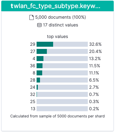
So what can we do now with this data that we couldn’t if we were streaming the pcap directly from the source into Elasticsearch? We can use the device names and a filter on whether the device is known or not (based on whether the MAC has an entry in the router’s internal table). Below is a useful illustration of the data. It shows, per device, the average signal strength during a period of time. Darker green means a stronger signal.
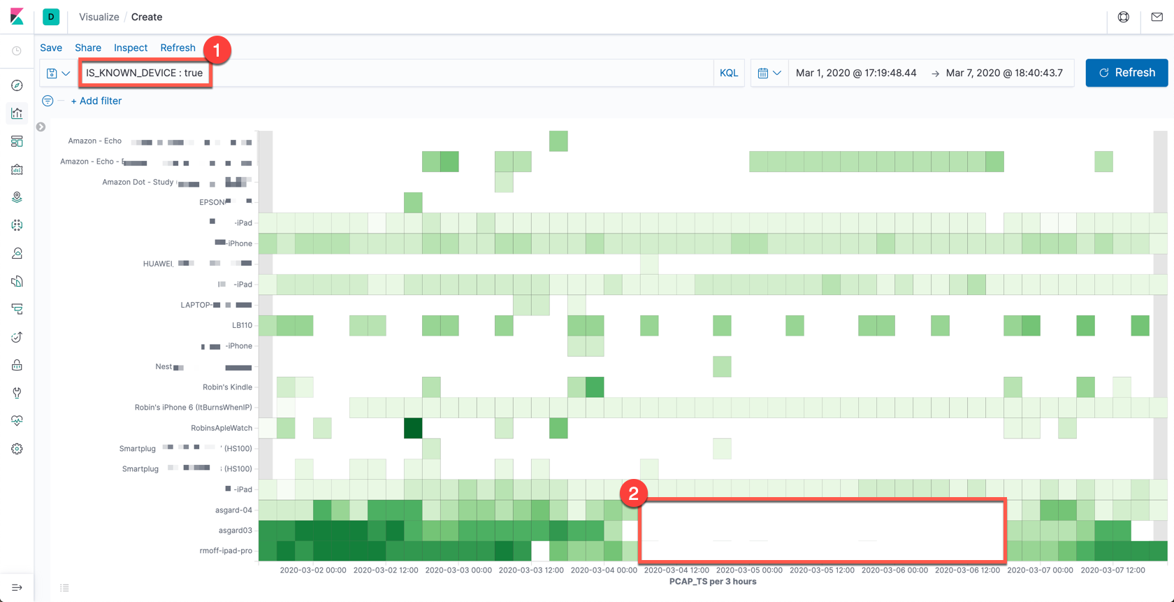
- We can accurately label all the devices and filter for ones which are known devices.
- There’s only data when a device runs a probe request—and if the device is absent, there’ll be no probes. The time period highlighted towards the bottom of the image corresponds to when I (along with my laptop, phone, and iPad) was away from home at a conference.
- You’ll also notice that the signal for the iPad and asgard03 devices (and to an extent asgard-04)—when present—is much stronger (darker green), because the devices are in the same room as the Raspberry Pi that is capturing the pcap data.
One of the things that I was interested to see was whether there was a discernable pattern in the data relating to the impact of the COVID-19 pandemic. Unfortunately, my test rig failed right around the time when the severe restrictions were put in place, but this is what the data looked like for the first three weeks of March:
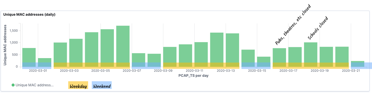
As discussed above, there’s a huge caveat to this data—tracking MAC addresses alone is not accurate because of MAC address randomisation used by many newer devices. You can read more about randomisation in this paper, but in essence, this is done deliberately for privacy reasons. By charting the data this way, we can dig into this randomisation a bit. Looking at the recent probe activity, I can see a relatively consistent number of probes, but a spike in the number of unique MACs on one of the days.
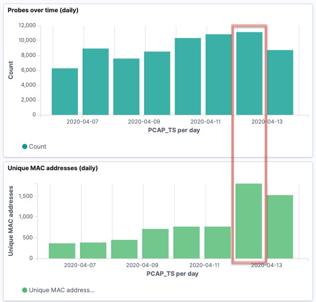
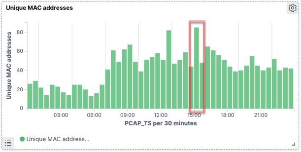
Drilling into that particular day, there’s a couple of spikes at specific points:
Taking a closer look, if we use a similar heatplot to the above data, we see that some devices (1) retain the same MAC address, therefore we see multiple probes over time from it at varying strength. In other cases, (2) we see signals of approximately the same strength (-69–-67, in orange on the image below) but with just single probes recorded.
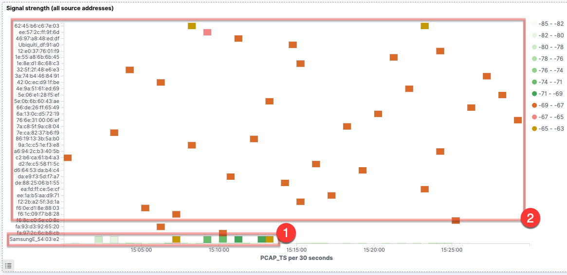
There are two scenarios that would account for the latter behaviour. The first is that there are multiple devices, each of a similar proximity to the device capturing the Wi-Fi probes, and each only sending a single probe request in the 30-minute interval. The second scenario involves a smaller number of devices, issuing multiple probe requests over time but changing the MAC address each time. Let’s see what else the data can offer to help us pursue these hypotheses.
By filtering the probe data for the signal range observed above, we get the following set of data, which reveals an interesting pattern:
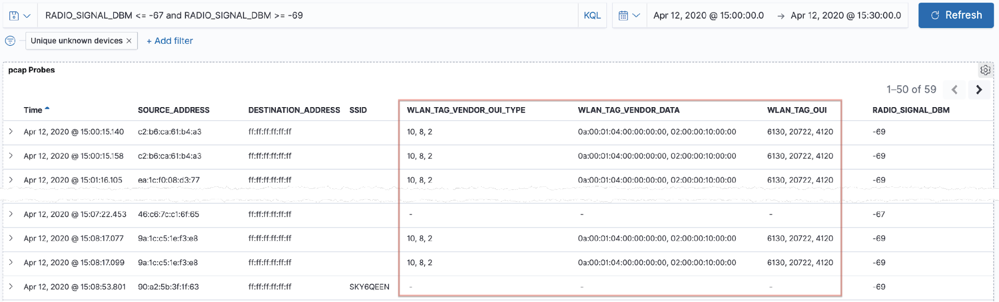
When devices send out probe requests, they include other data about the kinds of protocols that they support and so on. These fields (including wlan.tag.oui and wlan.tag.vendor.oui.type) are not unique to each device, but the combination of the values per packet forms a lower cardinality set than the probe results alone.
Looking at this set of probe requests, at the same signal strength and in the same time period, we see that almost all of them share the same set of wlan.tag.oui properties.
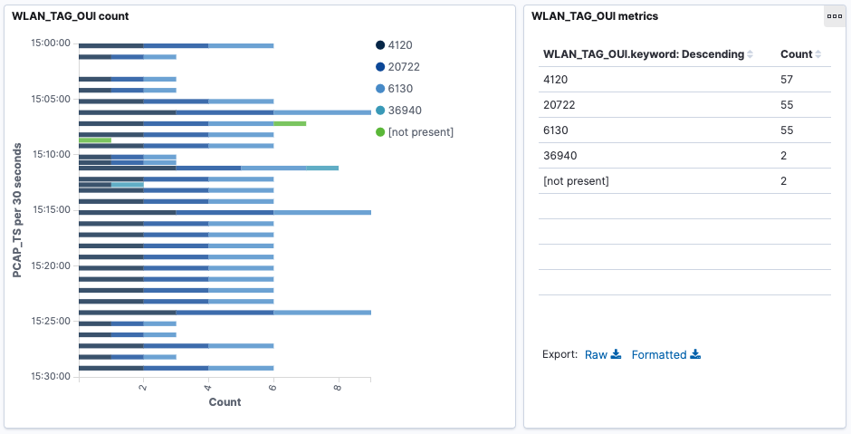
Using the manufacturer’s database from Wireshark, the Organizationally Unique Identifiers (OUI) can be decoded based on their hex representation:
- 4120 == 00:10:18 == Broadcom
- 20722 == 00:50:F2 == Microsoft Corp.
- 6130 == 00:17:F2 == Apple, Inc.
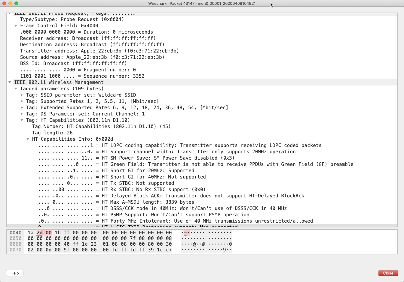
If you want to dig even further into this, the data that we’re streaming into Kafka can also be written to a local pcap file (add -b duration:3600 -b files:12 -w /pcap_data/mon0 to the tshark command to keep 12 hourly files of data). This pcap file can be loaded into Wireshark to see the real guts of the data that’s captured:
Wi-Fi probe pcap pattern matching with ksqlDB
The above analysis in Kibana showed how we can eyeball the data to explore and identify patterns of interest. But can we take a stream of data and automagically look for such patterns? Sure we can—with ksqlDB.
SET 'auto.offset.reset' = 'earliest';

CREATE TABLE OUI_FINGERPRINT_PROBES_01 AS
    SELECT WLAN_TAG_VENDOR_DATA,
           WLAN_TAG_VENDOR_OUI_TYPE,
           WLAN_TAG_OUI,
           COUNT(*)                                                    AS PROBE_COUNT,
           COUNT_DISTINCT(WLAN_SA[1])                                  AS SOURCE_MAC_ADDRESS_COUNT,
           COLLECT_SET(WLAN_SA[1])                                     AS SOURCE_MAC_ADDRESSES,
           TIMESTAMPTOSTRING(WINDOWSTART,'yyyy-MM-dd HH:mm:ss','GMT')  AS FIRST_PROBE,
           TIMESTAMPTOSTRING(WINDOWEND,'yyyy-MM-dd HH:mm:ss','GMT')    AS LAST_PROBE,
           (WINDOWEND-WINDOWSTART)/1000                                AS SESSION_LENGTH_SEC,
           MAX(WLAN_RADIO_SIGNAL_DBM[1])-MIN(WLAN_RADIO_SIGNAL_DBM[1]) AS SIGNAL_DBM_RANGE,
           HISTOGRAM(CAST(WLAN_RADIO_SIGNAL_DBM[1] AS VARCHAR))        AS SIGNAL_DBM_DISTRIBUTION
      FROM PCAP_PROBE
        WINDOW SESSION (5 MINUTES)
     GROUP BY WLAN_TAG_VENDOR_DATA,
              WLAN_TAG_VENDOR_OUI_TYPE,
              WLAN_TAG_OUI
    HAVING COUNT_DISTINCT(WLAN_SA[1]) > 2
    EMIT CHANGES ;
This uses a session window to identify probe requests matching this pattern:
- Identical set of properties (wlan.tag.oui, wlan.tag.vendor.oui.type, wlan.tag.vendor.data)
- Issued with a gap of no more than five minutes apart
- More than two different source MAC addresses
- Signal strength of all probes within 3 dBm of each other
All requests matching this pattern are grouped into a single result, from which we can see how many requests there were, which source MACs were used (and how many), the range of signal strengths, and so on:
SELECT ROWKEY AS FINGERPRINT,
       PROBE_COUNT,
       SOURCE_MAC_ADDRESS_COUNT,
       SOURCE_MAC_ADDRESSES,
       FIRST_PROBE,
       LAST_PROBE,
       SIGNAL_DBM_DISTRIBUTION
  FROM OUI_FINGERPRINT_PROBES_01
  WHERE WINDOWSTART > STRINGTOTIMESTAMP('2020-04-12 14:55:00','yyyy-MM-dd HH:mm:ss') AND WINDOWSTART < STRINGTOTIMESTAMP('2020-04-12 15:35:00','yyyy-MM-dd HH:mm:ss')
  EMIT CHANGES;
+---------------------+-------------+---------------------+---------------------+---------------------+---------------------+---------------------+
|FINGERPRINT          |PROBE_COUNT  |SOURCE_MAC_ADDRESS_CO|SOURCE_MAC_ADDRESSES |FIRST_PROBE          |LAST_PROBE           |SIGNAL_DBM_DISTRIBUTI|
|                     |             |UNT                  |                     |                     |                     |ON                   |
+---------------------+-------------+---------------------+---------------------+---------------------+---------------------+---------------------+
|[0a:00:01:04:00:00:00|16           |14                   | [6e:6f:18:05:08:16  |2020-04-13 14:21:56  |2020-04-13 14:45:03  |{-73.0=4, -71.0=11, -|
|:00, 02:00:00:10:00:0|             |                     | ,72:97:6c:9b:18:e9  |                     |                     |65.0=1}              |
|0]|+|[10, 8, 2]|+|[61|             |                     | ,7e:08:a9:8e:6c:79  |                     |                     |                     |
|30, 20722, 4120]     |             |                     | ,9e:89:88:d4:3f:64  |                     |                     |                     |
|                     |             |                     | ,7a:5f:3f:52:1d:ae  |                     |                     |                     |
|                     |             |                     | ,a6:ae:14:78:b4:6a  |                     |                     |                     |
|                     |             |                     | ,8e:2b:57:2a:e7:ff  |                     |                     |                     |
|                     |             |                     | ,86:d8:dc:50:aa:b0  |                     |                     |                     |
|                     |             |                     | ,8a:db:cf:ba:65:3a  |                     |                     |                     |
|                     |             |                     | ,5a:83:54:0a:4f:8c  |                     |                     |                     |
|                     |             |                     | ,62:d4:97:c2:ac:62  |                     |                     |                     |
|                     |             |                     | ,52:b2:39:e7:b1:cf  |                     |                     |                     |
|                     |             |                     | ,42:c4:7b:48:99:54  |                     |                     |                     |
|                     |             |                     | ,d6:5f:7b:35:0b:a6] |                     |                     |                     |
Analysing streams of data with ksqlDB
Let’s now take a step back from the nitty-gritty of Wi-Fi probe requests and randomisation of MAC addresses, and take a higher level view of the data we’re capturing. Using the enriched stream of data that was created from the live stream of packet captures joined to device information from my router, we can build a picture of all the devices that we see along with some summary statistics about them—when they last probed, which SSIDs they looked for, and so on:
SET 'auto.offset.reset' = 'earliest';
CREATE TABLE PCAP_PROBE_STATS_BY_SOURCE_DEVICE_02 AS
    SELECT CASE WHEN SOURCE_DEVICE_NAME IS NULL THEN
                SOURCE_ADDRESS_RESOLVED
            ELSE
                SOURCE_DEVICE_NAME END          AS SOURCE,
           COUNT(*)                             AS PCAP_PROBES,
           MIN(ROWTIME)                         AS EARLIEST_PROBE,
           MAX(ROWTIME)                         AS LATEST_PROBE,
           MIN(RADIO_SIGNAL_DBM)                AS MIN_RADIO_SIGNAL_DBM,
           MAX(RADIO_SIGNAL_DBM)                AS MAX_RADIO_SIGNAL_DBM,
           AVG(RADIO_SIGNAL_DBM)                AS AVG_RADIO_SIGNAL_DBM,
           COLLECT_SET(SSID)                    AS PROBED_SSIDS,
           COUNT_DISTINCT(SSID)                 AS UNIQUE_SSIDS_PROBED,
           COUNT_DISTINCT(DESTINATION_ADDRESS)  AS UNIQUE_DESTINATION_ADDRESSES
    FROM   PCAP_PROBE_ENRICHED
    GROUP BY CASE WHEN SOURCE_DEVICE_NAME IS NULL THEN SOURCE_ADDRESS_RESOLVED ELSE SOURCE_DEVICE_NAME END;
Under the covers, this aggregation is materialised by ksqlDB, which means that we can query the state directly:
SELECT SOURCE_DEVICE_NAME,
       PCAP_PROBES,
       TIMESTAMPTOSTRING(EARLIEST_PROBE,'yyyy-MM-dd HH:mm:ss','GMT') AS EARLIEST_PROBE,
       TIMESTAMPTOSTRING(LATEST_PROBE,'yyyy-MM-dd HH:mm:ss','GMT') AS LATEST_PROBE,
       PROBED_SSIDS,
       UNIQUE_SSIDS_PROBED
  FROM PCAP_PROBE_STATS_BY_SOURCE_DEVICE_02
 WHERE ROWKEY='asgard03';
+-------------------+------------+--------------------+--------------------+----------------------------+--------------------+
|SOURCE_DEVICE_NAME |PCAP_PROBES |EARLIEST_PROBE      |LATEST_PROBE        |PROBED_SSIDS                |UNIQUE_SSIDS_PROBED |
+-------------------+------------+--------------------+--------------------+----------------------------+--------------------+
|asgard03           |3110        |2020-02-28 22:51:22 |2020-04-14 11:06:13 |[null, , FULLERS, RNM0, loew|12                  |
|                   |            |                    |                    |s_conf, _The Wheatley Free W|                    |
|                   |            |                    |                    |iFi, skyclub, CrossCountryWi|                    |
|                   |            |                    |                    |Fi, QConLondon2020, FreePubW|                    |
|                   |            |                    |                    |iFi, Marriott_PUBLIC, Loews,|                    |
|                   |            |                    |                    | Escape Lounge WiFi]        |                    |
Query terminated
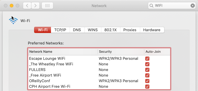
This query output is for my Mac laptop, and you can see that it is searching for various public and private networks. The names of these match those Wi-Fi networks to which my Mac has previously connected.
ksqlDB is proving pretty handy here. We’ve taken a raw stream of data, and using a couple of SQL statements, built a stateful, scalable aggregation that we can query in place from the ksqlDB prompt. We can also use the REST API to query it programatically, for example, to see when a given device last ran a probe:
$ curl -s -XPOST "http://localhost:8088/query" \
     -H "Content-Type: application/vnd.ksql.v1+json; charset=utf-8" \
     -d '{"ksql":"SELECT TIMESTAMPTOSTRING(LATEST_PROBE,'\''yyyy-MM-dd HH:mm:ss'\'','\''GMT'\'') AS LATEST_PROBE FROM PCAP_PROBE_STATS_BY_SOURCE_DEVICE_02 WHERE ROWKEY='\''asgard03'\'';"}' |jq '.[].row.columns'

[
  "2020-04-08 06:39:45"
]
If you want to see how I built on this idea of lookups against the materialised aggregation, be sure to check out Building a Telegram Bot Powered by Apache Kafka and ksqlDB.
And, of course, we can take the data that ksqlDB is aggregating for us and push it down to one or more target systems for further use and analysis:
- Elasticsearch
CREATE SINK CONNECTOR SINK_ELASTIC_PCAP_PROBE_STATS_BY_SOURCE_DEVICE_02 WITH (
  'connector.class'                             = 'io.confluent.connect.elasticsearch.ElasticsearchSinkConnector',
  'connection.url'                              = 'http://elasticsearch:9200',
  'topics'                                      = 'PCAP_PROBE_STATS_BY_SOURCE_DEVICE_02',
  'type.name'                                   = '_doc',
  'key.ignore'                                  = 'false',
  'schema.ignore'                               = 'true',
  'transforms'                                  = 'appendTimestampToColName',
  'transforms.appendTimestampToColName.type'    = 'org.apache.kafka.connect.transforms.ReplaceField$Value',
  'transforms.appendTimestampToColName.renames' = 'EARLIEST_PROBE:EARLIEST_PROBE_TS,LATEST_PROBE:LATEST_PROBE_TS',
  'key.converter'                               = 'org.apache.kafka.connect.storage.StringConverter'
);
- 'key.ignore' = 'false' means that it takes the key of the Kafka message (which is set in the CREATE TABLE above to the SOURCE field) and updates documents in place when changes occur in the source table.
- A Single Message Transform (SMT) is used to append _TS to the date fields. I created a document mapping template in Elasticsearch to match any field named *_TS as a date, which these two fields are (but stored as BIGINT epoch in ksqlDB).
- Postgres
CREATE SINK CONNECTOR SINK_POSTGRES_PCAP_PROBE_STATS_BY_SOURCE_DEVICE_02 WITH ( 'connector.class' = 'io.confluent.connect.jdbc.JdbcSinkConnector', 'connection.url' = 'jdbc:postgresql://postgres:5432/', 'connection.user' = 'postgres', 'connection.password' = 'postgres', 'topics' = 'PCAP_PROBE_STATS_BY_SOURCE_DEVICE_02', 'key.converter' = 'org.apache.kafka.connect.storage.StringConverter', 'auto.create' = 'true', 'auto.evolve' = 'true', 'insert.mode' = 'upsert', 'pk.mode' = 'record_value', 'pk.fields' = 'SOURCE', 'table.name.format' = '${topic}', 'transforms' = 'dropArray,setTimestampType0,setTimestampType1', 'transforms.dropArray.type' = 'org.apache.kafka.connect.transforms.ReplaceField$Value', 'transforms.dropArray.blacklist' = 'PROBED_SSIDS', 'transforms.setTimestampType0.type'= 'org.apache.kafka.connect.transforms.TimestampConverter$Value', 'transforms.setTimestampType0.field'= 'EARLIEST_PROBE', 'transforms.setTimestampType0.target.type' ='Timestamp', 'transforms.setTimestampType1.type'= 'org.apache.kafka.connect.transforms.TimestampConverter$Value', 'transforms.setTimestampType1.field'= 'LATEST_PROBE', 'transforms.setTimestampType1.target.type' ='Timestamp' );- Since the JDBC sink doesn’t support writing array objects to Postgres (you’ll get the error org.apache.kafka.connect.errors.ConnectException: null (ARRAY) type doesn’t have a mapping to the SQL database column type), we just drop it here using the ReplaceField SMT.
- The TimestampConverter SMT is used to set the type of the two timestamp fields so that they’re ingested into Postgres as timestamps (and not BIGINT).
- To get the rows to update in place as the source table in ksqlDB changes, 'insert.mode' is set to upsert. The primary key on the target table in Postgres is set to be built from the value of SOURCE (pk.fields) in the message value (record_value).
postgres=# \d "PCAP_PROBE_STATS_BY_SOURCE_DEVICE_02"
                 Table "public.PCAP_PROBE_STATS_BY_SOURCE_DEVICE_02"
            Column            |       Type       | Collation | Nullable | Default
------------------------------+------------------+-----------+----------+---------
 SOURCE                       | text             |           | not null |
…
Indexes:
    "PCAP_PROBE_STATS_BY_SOURCE_DEVICE_02_pkey" PRIMARY KEY, btree ("SOURCE")
Since SOURCE is also the record key in the Kafka message, you could use pk.mode = record_key here, but it would still need to be materialised onto the Postgres table. You’d end up with two fields in Postgres with the same value (SOURCE, plus whatever you set pk.fields to. In this context, it would be used by the connector as the name of the field in Postgres to store the Kafka message key in):
'pk.mode'             = 'record_key',
'pk.fields'           = 'PK',
postgres=# \d "PCAP_PROBE_STATS_BY_SOURCE_DEVICE"
                Table "public.PCAP_PROBE_STATS_BY_SOURCE_DEVICE"
            Column            |       Type       | Collation | Nullable | Default
------------------------------+------------------+-----------+----------+---------
 SOURCE                       | text             |           |          |
…
 PK                           | text             |           | not null |
Indexes:
    "PCAP_PROBE_STATS_BY_SOURCE_DEVICE_pkey" PRIMARY KEY, btree ("PK")

postgres=# SELECT "SOURCE","PK" FROM "PCAP_PROBE_STATS_BY_SOURCE_DEVICE";
      SOURCE       |        PK
-------------------+-------------------
 ea:28:50:4d:44:fb | ea:28:50:4d:44:fb
 12:c3:06:85:53:96 | 12:c3:06:85:53:96
…
(3 rows)
Graph relationships in the data
Phew. That was some deep stuff we did there with both Elasticsearch and Kibana for analysing and identifying patterns, and ksqlDB for building stateful aggregations of these patterns and general statistics on the data.
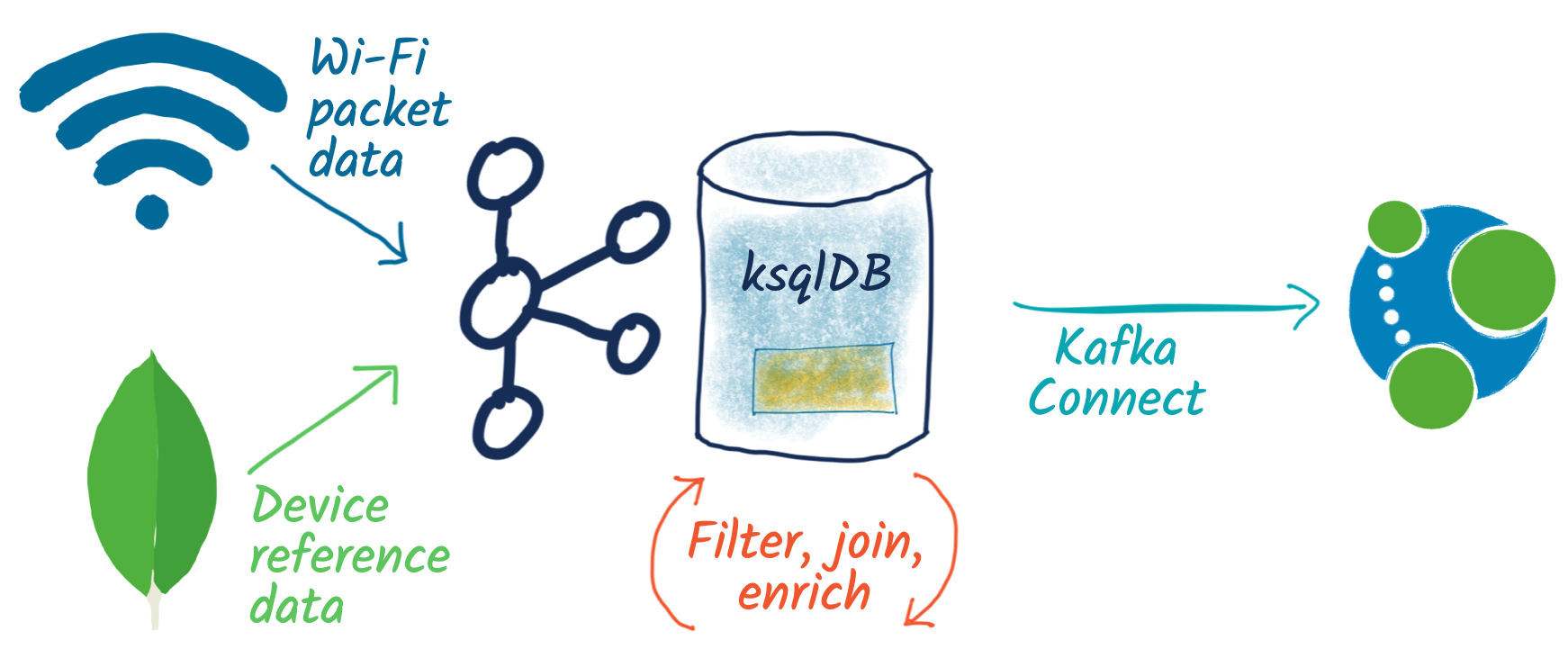
Let’s look at what else we can do with streams of data that we’ve got in Kafka. We’ll take the stream of probe requests that we filtered into its own topic and stream it to Neo4j:
CREATE SINK CONNECTOR SINK_NEO4J_PROBES_01 WITH (
    'connector.class'= 'streams.kafka.connect.sink.Neo4jSinkConnector',
    'topics'= 'pcap_probe_enriched_00',
    'neo4j.server.uri'= 'bolt://neo4j:7687',
    'neo4j.authentication.basic.username'= 'neo4j',
    'neo4j.authentication.basic.password'= 'connect',
    'neo4j.topic.cypher.pcap_probe_enriched_00'= 'MERGE (source:source{mac: event.SOURCE_ADDRESS, mac_resolved: event.SOURCE_ADDRESS_RESOLVED, device_name: coalesce(event.SOURCE_DEVICE_NAME,""), is_known: event.IS_KNOWN_DEVICE}) MERGE (ssid:ssid{name: coalesce(event.SSID, "")}) MERGE (ssid)<-[:LOOKED_FOR_SSID]-(source)'
);
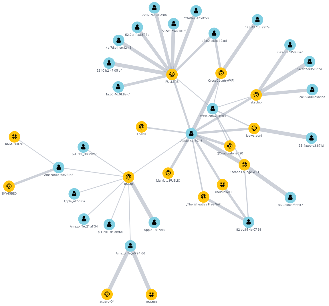
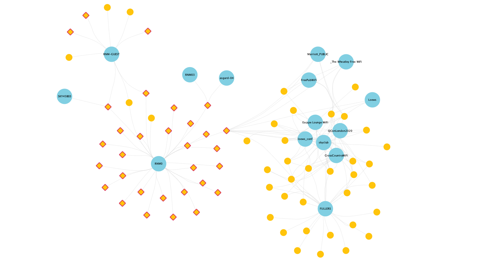
From here, we can really dig into the property graph: for example, relationships that exist between devices and the Wi-Fi networks (SSIDs) that they scan for. Below, we see my known devices (denoted by diamonds with red edging) scanning for my home Wi-Fi network, as well as a couple of these same devices also scanning for other public networks (pubs, airline lounges, train Wi-Fi, etc.), which other non-known devices also scan for:
You also get patterns like this, where some devices (yellow dots) have evidently connected to (and are thus scanning for) many networks, whilst others overlap only on common public ones (Northern-FreeWiFi is from the local train company; BTWiFi-with-FON is a shared Wi-Fi service).
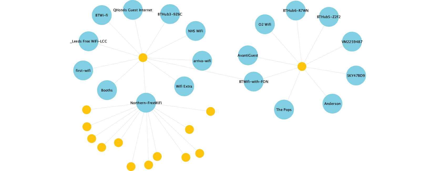
Other devices clearly just connect to one network only, ignoring all others.
Conclusion
Kafka is a great platform into which you can stream and store high volumes of data, and with which you can process and analyse it using tools such as ksqlDB, Elasticsearch, and Neo4j. Being able to create connectors from within ksqlDB makes it easy to integrate systems by both pulling data into Kafka and pushing it out downstream. Kafka provides a flexible platform on which you can process your data however you like, using the most appropriate tools for the task at hand. If you want to do complex property graph analysis, you can cleanse and prepare the data with ksqlDB and stream it to Neo4j. If you want to calculate rolling aggregates to drive an application or trigger alerts, you can build it directly in ksqlDB.
You can find the code for this article on GitHub.
Did you like this blog post? Share it now
Subscribe to the Confluent blog


