New in Confluent Cloud: Making Data & Pipelines Accessible for AI-Ready Streaming | Learn More
The Future of SQL: Databases Meet Stream Processing
SQL has proven to be an invaluable asset for most software engineers building software applications. Yet, the world as we know it has changed dramatically since SQL was created in 1974. In this article, you will learn how the future of SQL is being shaped by changes in how data is used to build applications. We’ll start with a brief history of SQL and how it’s been used with data systems through to the modern day and the rise of Apache Kafka®. We’ll then take a deep dive into several key areas where SQL—originally designed for data at rest—needs to meet data in motion so that we engineers can build the modern architectures that companies need today and in the future.
This blog post is part one of a series of Readings in Streaming Database Systems. Check out the other posts in this series:
- Overview: Readings in Streaming Database Systems
- Part 2: 4 Key Design Principles and Guarantees of Streaming Databases
- Part 3: How Do You Change a Never-Ending Query?
How SQL started
Over fifty years ago, when the first relational database was defined by Edgar Codd at IBM and SQL was created to interact with its tables of data, our world and its technology were tremendously different compared to today. That may sound like a somewhat trite observation, but just stop and think about it: Shops closed at 5 p.m. and didn’t open on Sundays (in Switzerland and the UK, anyway). If you wanted to buy something without going to a shop, you could use a mail order catalogue and get it several weeks later, after posting a cheque in the post. In hospitals, sensor readings were all done analogue and manually, instead of electronically and automated. Our beloved smartphones and mobile Internet were decades away.
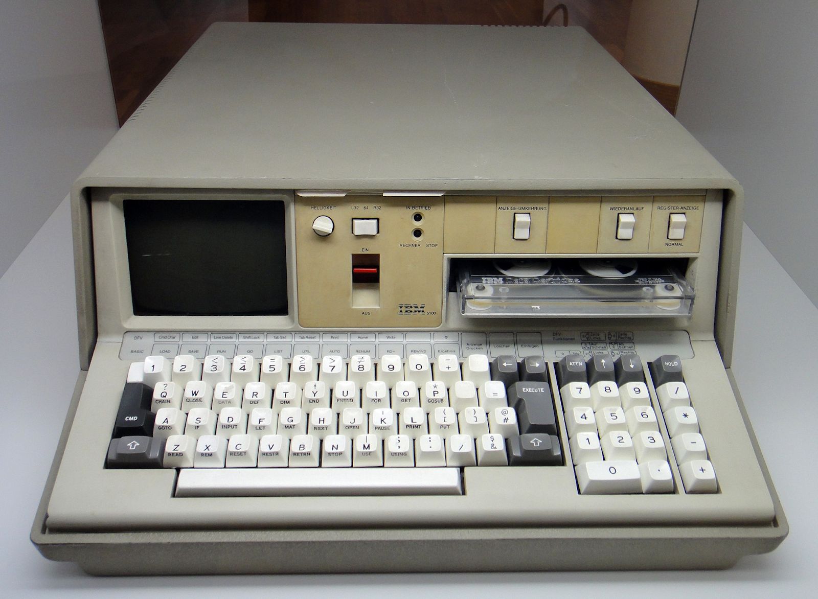
The “portable” IBM 5100 from 1977, introduced a few years after SQL was created. Fast forward to today, where we are continuously creating and consuming much more data with much more powerful computers that fit into our pockets.
Source: IBM 5100 computer (1974), Swiss German keyboard and markings.
Even in these early days of software and data, the relational database and SQL were destined to thrive and take both the software industry and computer science academia by storm over subsequent decades.
The relational database was essentially designed to work with a singular shared data set, and to fulfill business logic by serving queries and computations on the shared data set, making humans more productive. By providing the ability to process and store huge amounts of information, many tasks, such as inventory management or financial accounting, could be done in a fraction of the time previously needed to do them manually. The rise of SQL throughout all of this foreshadowed the importance of being able to work with data in a way that is simple and easy.
How SQL is used today
Our world today is remarkably different from 1970. People, devices, and businesses are online all of the time, and they are generating and consuming data all of the time. All of this data never rests! We do not work with a singular, shared data set anymore, but with data that flows from and to many different places, and wherever it is flowing to, it is driving computation in our applications and business logic. And while the original usage patterns are still relevant, we as engineers are being tasked with solving much more demanding use cases: we are building infrastructures where software is predominantly talking to other software: machines that interact automatically and 24×7 with other machines. In today’s world, data is always in motion, and our infrastructures need to process these streams of data immediately. The trusty relational database and SQL weren’t designed for this futuristic world.
In 2009, Apache Kafka was created by the future founders of Confluent, and it has since become the de-facto technology by which thousands of companies today are creating, collecting, storing, and processing data in motion—with streams of events, using stream processing. Yet the overall developer experience for data in motion has still been quite a bit off from what we’re used to when writing a simple, declarative SQL statement in a relational database for working with data at rest. What will it take to make this world more serviceable by today’s databases?
What we need are new language abstractions and query semantics for solving these new use cases, because they need to operate on both data in motion and data at rest. Current databases have only solved one half of it—they give us tables for data at rest. In the subsequent sections, we will highlight the key areas of what we believe needs to be added to SQL to make the database more complete. To make the examples more concrete, we’ll be using ksqlDB, a streaming database that was designed from the ground up for both data in motion and data at rest, to illustrate these key areas.
Tables only tell half of the story
Relational databases were designed to store the current state of the world in the form of tables, and to answer questions about this state via point-in-time queries against the tables: “What is Alice’s account balance right now?” Even if there are a few extensions in SQL such as temporal tables, there is still a big gap between the table state itself vs. how the state was computed over time. In other words, there is no way to determine from a table alone how that state originated—think: “How did we get here?”
This is where streams come into play. Event streams model the world around us. By storing individual data records (events) non-destructively as an ordered sequence—the proverbial log data structure that every software engineer should know about—they provide a detailed historical view of what happened. This history—of both human and machine-generated events—can be replayed for processing and reprocessing. Not only that, but event streams provide the original facts (Alice received $10, then Alice received $20) from which table state can then be derived (Alice’s current balance is $30). Contrast this to traditional databases, where they can only give you access to whatever happens to be the current table state.
Here’s an analogy to playing chess: If you have a recording of all the moves on the chessboard, it is straightforward to know what the current state of the board is. You can also easily rewind the time, using the recorded stream of moves, to know all of the historical states of the board.
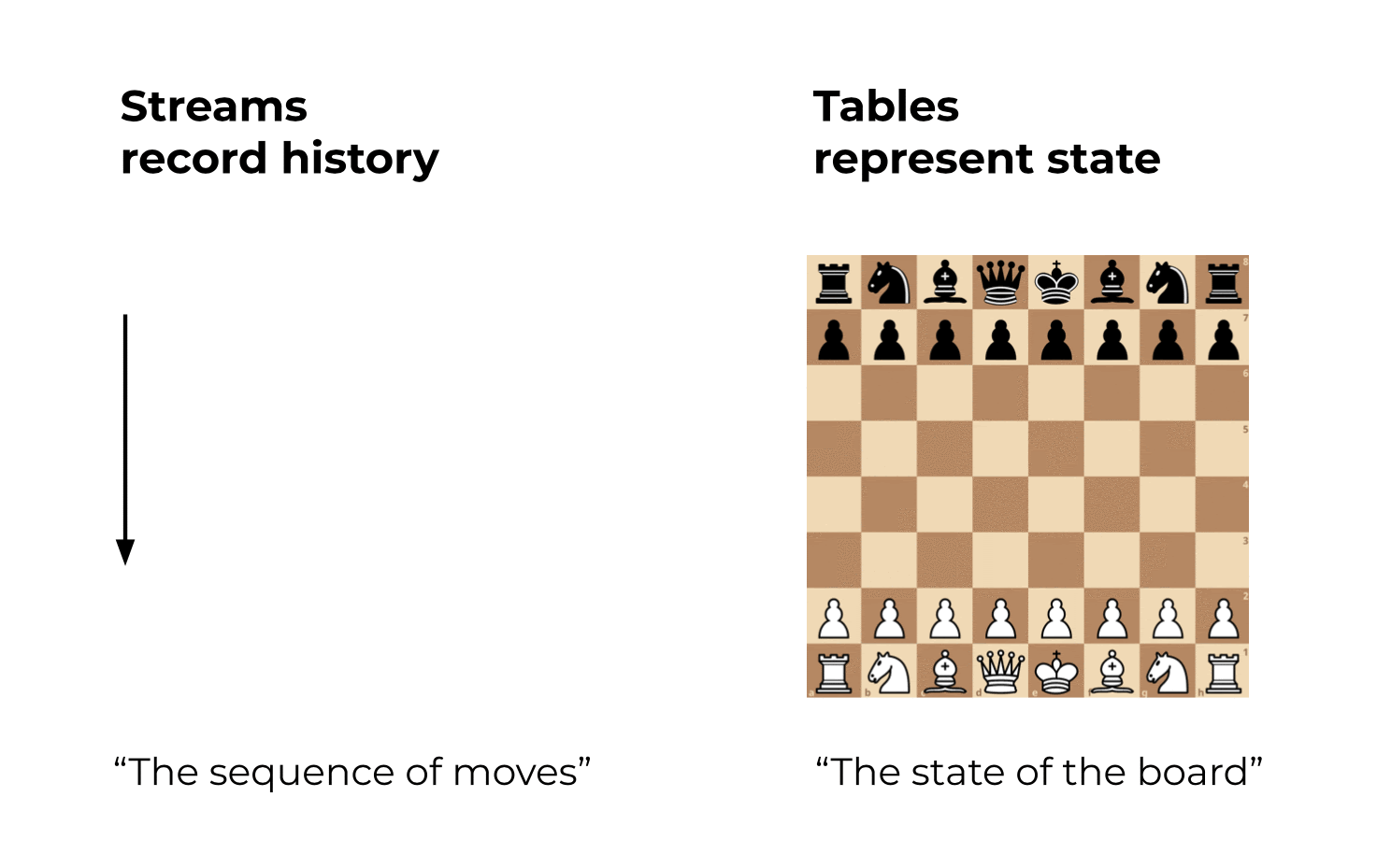
Figure 1: Streams record history. Tables represent state.
To work with data in our systems we need both streams and tables. But so far, technologies have supported one or the other, forcing a wedge between what are two naturally complementary ways of handling data. We could either have state, or we could have events, despite the many benefits of being able to use the semantics of both in one place. What are those benefits? Let’s consider an example. As a bank, you can model the stream of payments from customers as a stream. You’ll want to store this stream for many years—you might even be required by law to do so. From this stream, you can write queries that derive a table of each customer’s account balance. Because the table is built on a stream, it will continually update and so you will always have a current view of the state of the world (your customers being your world here). Not only can you build a table of customer account state, but you can also build further tables to segment it by customer group, country, etc.
To model these two different but very related concepts, a system needs to support two first-class data constructs:
Let us now examine these constructs in more detail and think about the enhancements to existing SQL that might be needed.
Adding a STREAM abstraction to SQL
As we have discussed above, processing data in motion and processing data at rest imply different semantics. For example, data streams are inherently ordered by time, because they represent events that happen one after another. In contrast, tables model the current state of the world, i.e., everything that is true at the same time.
Supporting streams as a first-class concept in SQL gives us the ability to model our queries and processing semantics more accurately. It’s completely appropriate to query a stream of events, but to call that stream a table (per SQL’s current model) is like trying to force a square brick into a round hole.
For example, if we are interested in all of those orders that have been shipped, and we also want to include any orders in the query result as soon as their status changes to “shipped”, we can run this query:
SELECT * FROM orders WHERE status=‘shipped’ EMIT CHANGES;
The above query “tails” the stream of orders and adds a new result record whenever an order status changes to “shipped”. We will discuss more details about streaming queries later in this post.
Sidenote: Streams can be tables too!
As well as modelling a Kafka topic as a stream of data as detailed above, a streaming database like ksqlDB allows us to also model a Kafka topic as a table. It’s even possible to define a stream and a table for the same input topic: in the end, it’s just different semantic interpretations of how you want to use the data. Kafka has built-in support to model streams and tables with its different topic cleanup policies: “delete” and “compact”.
Using our chessboard example, you might be interested in how often the queen was moved, but you might also want to know its current position: ksqlDB can answer both questions based on the same underlying data. Furthermore, a stream can be aggregated into a continuously updated table (or materialized view) to “roll up” events into a more compact representation of the data (we will discuss this use case in more detail later).
Query types in a modern database
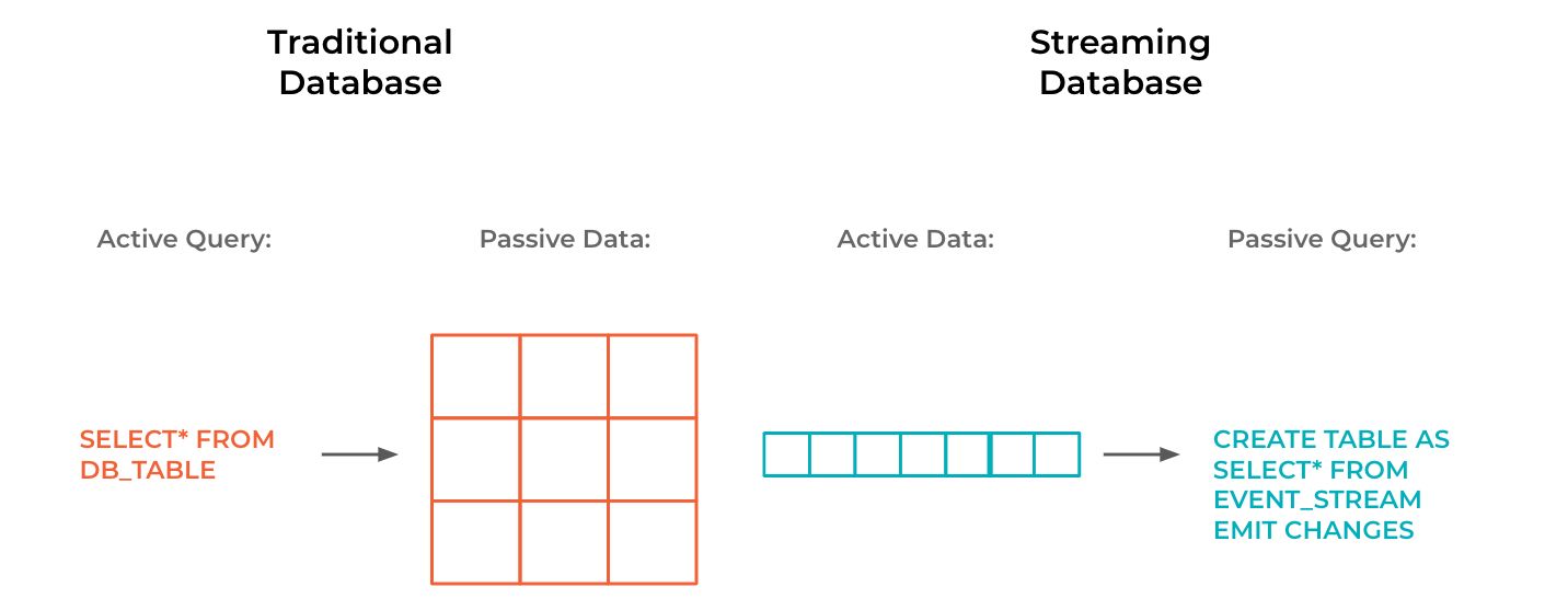
SQL is a powerful language that allows us to express complex questions of our data with ease. In a traditional database, there is a “data-passive, query-active” approach. Data sits at rest in the database until the user issues a query to add or retrieve a piece of data. If the data in the database changes, the user has to re-issue the same query to get an updated result (or rely on functionality such as triggers).
In today’s world, this approach alone does not fulfill the whole paradigm in which we want to interact with data. We are increasingly building architectures in which systems drive other systems directly. And this requires a change of strategy: The modern database must support a “data-active, query-passive” approach in which queries execute and passively wait for new data to arrive from upstream queries and data sources.
The advantage of this design is that each newly arriving data record will cause the query to immediately process and react to the new information. Any data changes are now quickly being propagated throughout the entire system. Achieving this requires the introduction of new query types, which we cover in the next section.
A new query type for streaming SQL
In a traditional database, data is at rest, and we can query it to find out the state at the point at which we run the query. If we want to know if that state has changed, we re-run the query. The state we are interested in could be a customer’s address, or it could be an analytical query perhaps telling us how many tins of beans we’ve sold so far in a given time period. Either way, we need to run the query each time we want a current answer. We can think of this as “pulling” the data from the database, as opposed to “pushing” (this is covered further in the next section). As the volume of data increases, and the frequency with which we receive it goes up too, this approach of simply re-querying a database as the data changes becomes inefficient, poorly performing, and simply not in keeping with how we should actually interact with the data.
A more natural—and more efficient—match for streams of data is to run streaming queries. Here, the database performs stream processing in which results are computed continuously, one event/record at a time. These results are then pushed into a new stream of events. This allows us to subscribe to query results.
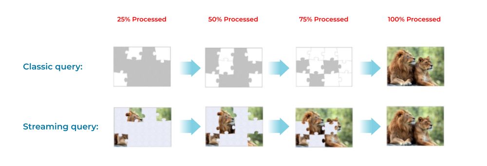
Streaming queries are for data in motion, whereas classic “point-in-time” queries are for data at rest. To make an analogy, processing a database query is a bit like solving a puzzle. With a classic query, we can only see the face of the puzzle (the final query results) after all the pieces (the data) fit together. With a streaming query, we can see the face as it evolves.
What does this mean for the SQL grammar? Even in newer databases, there’s no reason to change the syntax for a classic (“pull”) query from what we’re used to with any existing RDBMS. For example, we can still lookup rows in a table of customers with:
SELECT * FROM customers WHERE country = 'Italy';
However, to run streaming (“push”) queries, we need a new way to indicate to the database that it is to provide a stream of the result changes, and we do this by using the EMIT CHANGES suffix:
SELECT * FROM customers WHERE country = 'Italy' EMIT CHANGES;
Note that the SQL statement of this push query is almost identical to the pull query before, with the exception of the EMIT CHANGES clause. The important difference lies in the query behaviour:
- The push query keeps running forever until it is explicitly terminated. Contrast this to a pull query, which terminates once the (bounded) result has been returned.
- The result of the query is an unbounded change stream: each time the data for a customer changes (including DELETEs and INSERTs), a new result record is sent to the client.
Pull vs Push queries: Differences in execution
Let’s look at how these two different query models work in practice, taking a simple customers table and a query against it looking for any customers in Italy.
In a regular RDBMS, a query requires a full table scan every time it is run (unless you put an index on the country column). And, since there are no push queries in traditional RDBMS systems, clients need to re-submit the same query periodically to learn about any changes to the data.
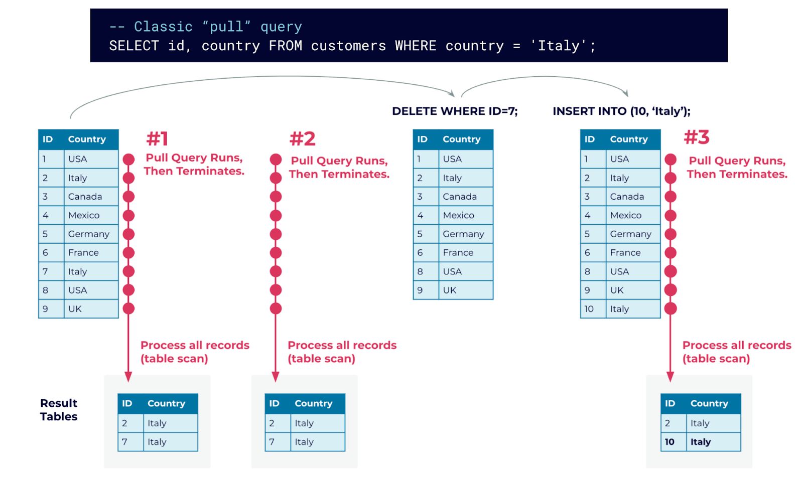
Figure 2 (a): Using three classic queries to query a table at different points in time. Results are computed from scratch by each query.
Figure 2 (a) shows our customers table as it changes over time. We execute a pull query three times against the table, at different points in time. Note that nothing changed on the input table when the query is executed the second time, while the two updates to the table are only “detected” when the query is executed the third time. Hence, we had to perform a full table scan without getting a new result, which is wasteful. Secondly, it results in increased latency to learn about the DELETE of the row with ID=7.
In contrast, a push query can be computed quite efficiently as shown in Figure 2 (b). On query submission, a single table scan is performed to return the initial query result. But afterwards, the still running query only needs to subscribe to changes to the customers table, i.e., individual INSERTs, UPDATEs, and DELETEs.
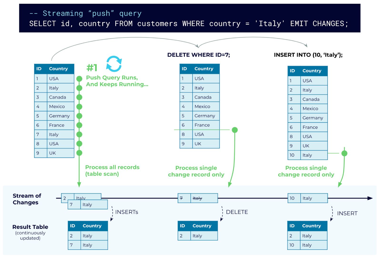
Figure 2 (b): Using a single streaming query to subscribe to table changes. Results are computed incrementally with stream processing.
This “subscription for changes” is very efficient in streaming systems like Kafka and ksqlDB. Thus, instead of paying the cost of a full table scan again and again, the cost to compute “deltas” (i.e., to incrementally compute subsequent result records of the query) is no longer linear in the full table size O(number of records in input table), but only linear in the update frequency of the table O(rate of table changes). If no table updates happen, nothing needs to be computed and there is almost no overhead. And if an update does happen, the result delta (if any) is pushed to clients immediately. This reduces the end-to-end latency to inform the clients about the change, ensures that clients do not miss any updates, and makes the preemptive rerunning of queries an obsolete pattern.
Building materialized views on a stream of data with persistent queries
When a client executes a query, that query is transient. Even if it is a push query and the client receives multiple results over an unbounded period of time, the query terminates once the client disconnects. This mirrors what happens in an RDBMS.
However, since events may continue to arrive on a stream, why should a streaming database only process those events when a client is connected? That is why we have a new type of query: the persistent query. These queries are continuously executed in the servers of the database cluster without any client interaction, and they write their results into a stream or table inside the database. A persistent query (a form of a continuous query), continually updates the target stream or table as new input data arrives.
For example, the following persistent query reads the payments stream to build a materialized view as a result table called balances that contains the latest balance per credit card number:
CREATE TABLE balances AS
SELECT card_number, SUM(amount) AS balance
	FROM payments
        GROUP BY card_number
	EMIT CHANGES;
Every time a new payment event is appended to the input stream, the event will propagate through the query, and the respective balance in the table will be updated automatically. If multiple queries are reading from the same stream or table as input, any change to the inputs will propagate through all of those queries. Furthermore, the result of a persistent query may be the input to another persistent query, and thus updates might propagate through a deep topology of persistent queries, updating all of their results.
Recap
In a streaming database like ksqlDB, we distinguish between two main categories of queries:
- Classic queries for table lookup (aka “pull queries”)
- Continuous streaming queries
We further subdivide streaming queries into (a) transient subscriptions (aka “push queries”) that continuously send new result records to a client and (b) persistent queries that run inside the database server and continuously update a result STREAM or TABLE (i.e., materialized view) whenever new input data becomes available.
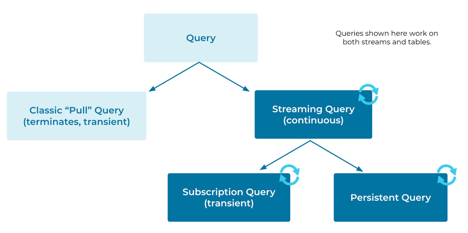
Figure 3: Query types in a streaming database.
Figure 3 above depicts the query taxonomy and shows the three different query types:
- Classic “pull” queries
- Subscription queries
- Persistent queries
New SQL syntax for STREAMs
Adding a STREAM to SQL raises the question on “how do I query a stream”? We showed a few examples already and will cover the key extensions in this section.
Temporal query semantics
Time is a foundational concept in stream processing. An event, whether machine- or human-generated, occurs at a particular point in time. The evolution of the world around us can be modelled as events, which progress forwards in time.
Querying a stream should provide results based on time, which is not only surprisingly challenging, but also extremely important. In practice, it’s quite possible that an event may arrive at the processing system much later than when it originally occurred at its source and thus lead to unorder in the data stream. This could be due to the source of the data (such as on an unstable mobile network) or unforeseen system problems upstream.
It’s beyond the scope of this blog post to deep dive into how a streaming data archives temporal query semantics, but the central cornerstones are:
- An event timestamp for every record (exposed a ROWTIME in ksqlDB)
- The notion of stream-time: a logical event-time base timeline that allows the streaming database to reason about processing progress
If you are interested in some more details about time semantics in ksqlDB and Apache Kafka, you might be interested in the following Kafka Summit talks:
Windowing for aggregations
In the example of the balances table above, we aggregate the full data stream into a table. However, a common requirement is to aggregate events based on time. All events include event time, and we can use this to aggregate streams over time-intervals. To do this, we need to introduce new syntax to SQL to be able to describe these time-windowed aggregations.
In the example below, we compute the credit card balance per week from the payments stream, with event-time processing semantics:
CREATE TABLE weekly_balance AS
  SELECT card_number, windowStart, SUM(amount) AS balance,
         MIN(payment_ts) AS first_payment,
         MAX(payment_ts) AS last_payment, COUNT(*) AS payments_ct
  FROM payments
  TUMBLING WINDOW (SIZE 1 WEEK, GRACE PERIOD 1 DAY, RETENTION 1 MONTH)
  GROUP BY card_number;
An oversimplification of the TUMBLING WINDOW clause is to think of it as an additional grouping condition along the timeline of data records: the aggregation SUM(amount) is not performed over all of the transactions per card number, but further divided per card number, into 1-week time “buckets” (i.e., windows), and a new row is added to the result table per card number and window. However, defining a window is more than just grouping:
- Groups are distinct and thus each record belongs to exactly one group. However, windows may overlap and thus a record can belong to multiple windows.
- Groups don’t have time semantics and they are always “open” while time progresses. However, windows are closed at some point while time progresses and won’t accept any more records afterwards.
- There are the additional time-related clauses RETENTION and GRACE PERIOD.
Discussing all details of windowed semantics is beyond the scope of this blog post, but if you’d like to dive into it please refer to the Kafka Summit talk The Flux Capacitor of Kafka Streams and ksqlDB. Ultimately, it comes down to the business requirements to resolve the trade-off between query execution cost (how much result history to store), result latency (how long to wait until publishing a result), and result completeness (if a window is closed too early, input data might be missed).
Streaming joins
Joins are very powerful and allow you to stitch together data from multiple data sets, enrich data, and discover correlations. Joining unbounded streaming data is equally (or even more?) powerful as we will discuss in this section.
Enriching the JOIN clause for stream-stream joins
Streams are conceptually infinite and thus joining two streams implies potentially joining all events of both input streams. Generally, this would require infinite storage because we can never safely drop an event as it might join with a future event from the other stream. To tackle this issue, ksqlDB reuses the idea of a windowed computation and introduces the WITHIN clause. This applies a sliding window to the join so that the join becomes bounded:
CREATE STREAM joined AS
   SELECT *
   FROM left_stream AS l INNER JOIN right_stream AS r
         WITHIN 5 MINUTES GRACE PERIOD 30 SECONDS
         ON l.someAttribute = r.otherAttribute;
Similar to the TUMBLING WINDOW clause in aggregation, the WITHIN clause could be read as an additional join condition on the event-timestamps of input records. However, the WHERE clause approach has certain disadvantages:
- Bad user experience (i): This approach is error-prone because a user could forget to add the required time constraint, causing the query to eventually fail because it will run out of memory
- Bad user experience (ii): Just as expressing the key relationship in the ON clause of a join aids readability of the query (and thus eases future maintenance), so also does keeping the time semantics of the JOIN in the clause
- Insufficient semantics: We cannot express additional time-related concepts, such as a GRACE PERIOD
Note that a stream-stream join gives you real-time results: each time a new event appears on either input stream, it would flow through the continuous streaming query and try to find join partners in the window of the other stream. If any join partner is found, the join result is appended to the result stream immediately. This behaviour is quite different from relational table-table joins, which are usually very expensive and provide results often with high latency.
Stream-Table joins: Event-by-event attribute lookups
Joining data streams in real-time is one application of a streaming join. A second application is to join events in a stream to rows in a table in order to enrich the events with additional information. The following example statement illustrates this setup:
CREATE STREAM enriched_payments AS
	  SELECT *
	  FROM payments INNER JOIN customers
               ON payments.customer_id = customers.id;
Note that the result of this query is a stream (per the CREATE). For each customer transaction, the stream-side payment event is used to do a lookup into the customer table to enrich the event with the corresponding customer information, and the enriched event is appended to the result stream:
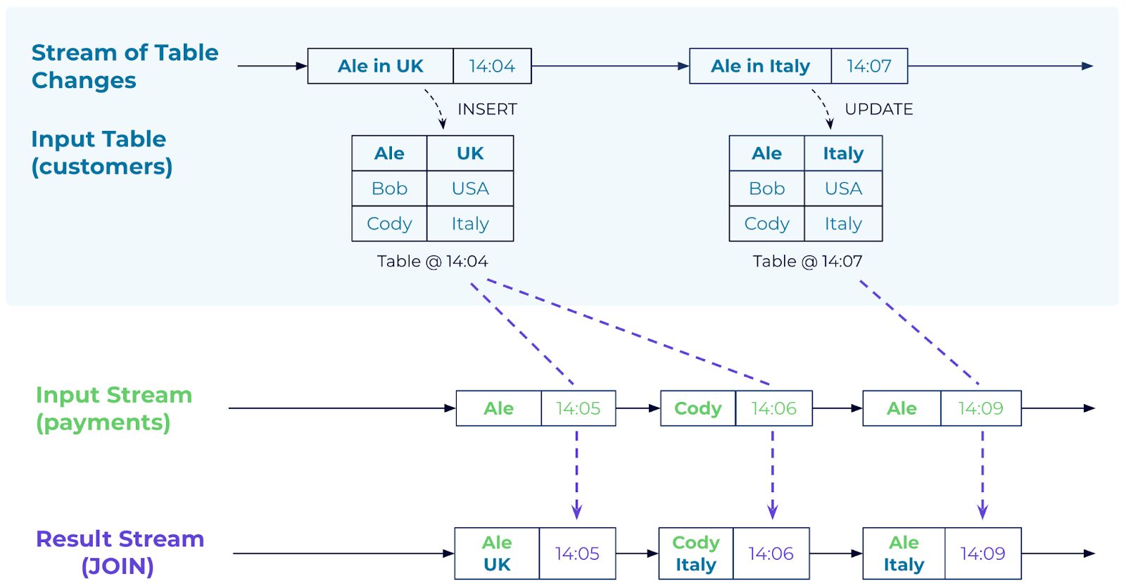
Figure 4: Joining a stream to a table. Alice’s payment in the stream at 14:05 is enriched by joining it to the customer table’s corresponding “version”. At 14:05, Alice was still in the UK.
Similar to a stream-stream join, results are provided in real-time. Each time a new event appears on the input stream, it flows through the query to perform that table lookup, and the enriched event is appended to the result stream right away.
Also note, that the table may be updated while the query is running: for this case, updates to the table are time-synchronized, and only newer events will see those changes. Already enriched events won’t be updated if the table changes, to ensure immutability.
Summary on joins
In a streaming world, we extend joins to not only allow table-table joins, but we also allow for real-time stream-stream and stream-table joins. Both joins offer new join semantics compared to relational table joins, and these operations provide natural semantics for data in motion use cases when compared to similar operations designed for data at rest.
If you want to learn more about streaming joins, you can check out the Kafka Summit talk Temporal Joins in Kafka Streams and ksqlDB.
Extending SQL beyond processing: Streaming ingest and egress
If data in motion wants to stay in motion, then this means the streaming database needs to offer a broad set of options to integrate data across system boundaries. In the previous sections, we already covered push queries, an enhancement of SQL that lets applications subscribe to query results as data in motion. However, what is also needed is the ability to integrate with external systems, including cloud services, in a way that keeps the data in motion: to continuously import and export data streams. With this functionality, we can then implement end-to-end use cases with a streaming database that leverages our existing investments, like a mainframe, a self-managed Oracle database, and cloud services such as AWS S3, Datadog, and MongoDB Atlas. In comparison, classic databases are focused on data at rest, and their functionality to connect to and share data with other systems is often limited and often supported only by out-of-band tooling.
Figure 5: Data in motion wants to flow across applications and systems, as shown in this screenshot of Confluent Cloud.
To integrate with external systems, ksqlDB leverages Kafka connectors: With the CREATE CONNECTOR statement, you can define source connectors to import data from external sources as streams, and you can define sink connectors to export data as streams to external destinations. In some sense, you can think of this functionality also as “real-timing” your existing systems, such as your trusty mainframe.
CREATE SOURCE CONNECTOR `customers-from-postgres` WITH (
    'connector.class' ='io.confluent.connect.jdbc.JdbcSourceConnector',
    'connection.url'  ='jdbc:postgresql://localhost:5432/my.db',
    ...
    'mode'            = 'bulk',
    'topic.prefix'    = 'jdbc-',
    'table.whitelist" = 'customers',
    'key'             = 'customerid');
The example above continuously imports data from Postgres into ksqlDB. The example below continuously exports from ksqlDB to Elastic.
CREATE SINK CONNECTOR `orders-to-elastic` WITH (
    'connector.class' = 'io.confluent.connect.elasticsearch.ElasticsearchSinkConnector',
    'connection.url'  = 'http://elastic:9200',
    'type.name'       = 'kafka-connect',
    'topics'          = 'orders');
Design-wise, it was a natural choice to use Kafka’s existing Connect framework for this purpose in ksqlDB, as Kafka Connect has been battle-tested in production for many years, and there is a vibrant ecosystem and community that provides hundreds of ready-to-use connectors.
Summary
In this blog post, we discussed why the database world needs three enhancements to the SQL language to support a complete handling of both data at rest and data in motion. These include:
- A new STREAM abstraction
- New query types like continuous and persistent queries
- Extended semantics for handling time
We used ksqlDB as the running example to illustrate what this looks and feels like in practice, such as for computing continuous aggregations and joins.
To foster broader adoption of stream processing, we also believe in incorporating Streaming SQL functionality into the official SQL standard. And fortunately, there is progress being made on this front as we speak! Confluent is an active participant in INCITS, the U.S. national body for these standard discussions. Specifically, we are working in the technical committee DM32 (Data Management and Interchange) that develops standards for database languages and metadata, which includes the SQL standard. Here, we are collaborating in a Streaming SQL working group together with vendors of traditional databases such as Microsoft, Oracle, and IBM, but also vendors of stream processing systems like Google and Alibaba. This list of participants, many of which are industry leaders with both technical pedigree as well as strong market reputation, also presents a clear validation of the increasing importance of event streaming and streaming databases in modern software architectures.
Although ksqlDB has a strong feature set today, completing its larger vision of marrying databases and stream processing remains an ambitious work in progress. We have certainly not yet reached the end of the language evolution journey, and at Confluent we are excited and humbled to collaborate with other industry leaders to the future of the SQL standard with event streaming.
If you’re interested in using ksqlDB, get started today via the standalone distribution or with Confluent, and join the community to ask a question and find new resources.
Other posts in this series
Did you like this blog post? Share it now
Subscribe to the Confluent blog


Why ELT Can't Keep Up in the Era of High-Scale Data Engineering
Batch ELT pipelines create duplication, cost spikes, and governance gaps as data scales. Here’s why enterprises are rethinking legacy integration models.


How to Protect PII in Apache Kafka® With Schema Registry and Data Contracts
Protect sensitive data with Data Contracts using Confluent Schema Registry.