[Webinar] How to Implement Data Contracts: A Shift Left to First-Class Data Products | Register Now
Data Enrichment in Existing Data Pipelines Using Confluent Cloud
If you are new to Apache Kafka®, this article is a great way to help you kick-start your first Kafka project and set your data in motion. The best way to learn a technology is to extend an existing project, because you have a clear picture of what a complete project has to have.
With that in mind, this blog extends the real-time houseplant alerting project built by Confluent’s Danica Fine to show you how to piggyback on an existing project using Cluster Linking, how to produce and consume events in Kafka, and how to manipulate real-time streaming events with ksqlDB, a database built for streaming purposes.
You are encouraged to read the original project blog post if you haven’t done so already. In a nutshell, the plant project captures soil data from houseplants, such as temperature and moisture level, and produces the real-time streaming data to Kafka. From there, a ksqlDB application determines when a given plant’s moisture level falls below a specific threshold deemed risky for that species, and, finally, Kafka Connect captures the low moisture events and sends them directly to Danica’s smartphone through Telegram, alerting her to water her plants.
This project is straightforward to understand. Plus, the extensibility of Confluent provides the opportunity to expand the project. With Cluster Linking, the existing soil readings can be moved to another Confluent Cloud cluster where real-time weather data from the houseplants’ locations can be integrated to see if weather humidity is a crucial factor that affects the soil moisture for each plant.
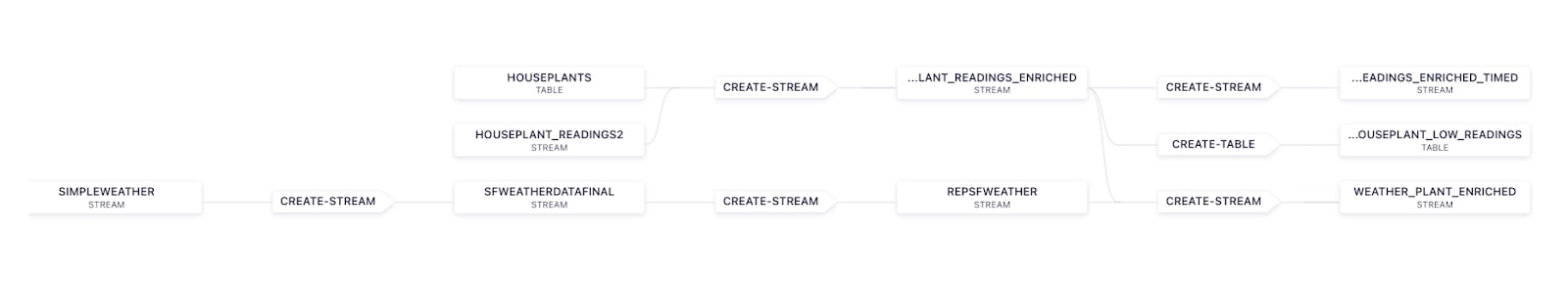
The graph below shows a high-level structure of the project:
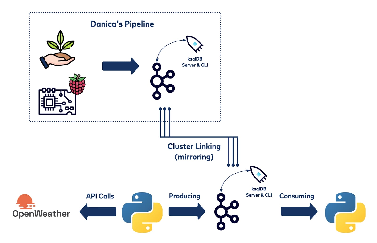
To begin, this project first clones the houseplant readings data stream using Cluster Linking. From there, a Python application is created to pull data from openWeather’s API and produce each message to a topic on Confluent Cloud.
The main goal of this project extension is to show new users to Kafka or Confluent Cloud how accessible and beginner-friendly Kafka is. It walks you through how to build this data pipeline in detail, from capturing the weather data from a free public API, appending data to Kafka topics, filtering and joining data streams via ksqlDB, consuming data from client applications, and training a simple linear model.
Accessing Source Data
To extend the project, the first step is to gain access to the source readings data being captured by the Raspberry Pi. Unfortunately, I don’t have direct network access to the Raspberry Pi. So how do you get access to the readings data within your own cluster? The houseplant alerting system had been running for months, meaning that a long history of plant moisture data had been persisted to the source cluster. This is where Cluster Linking comes in.
Cluster Linking is an excellent technology that allows users to mirror topics from a source topic to a destination topic even though the two clusters may be hosted in different locations. It not only provides a great way for sharing topics and expanding existing projects, it also provides some resilience by replicating topic data and metadata to another cluster with low latency and ensures minimal data loss at the same time.
Using Cluster Linking, I linked Danica’s cluster with mine and mirrored exact messages—byte for byte, offset by offset—from specific Kafka topics from one cluster to another. This includes both the previously generated data and all future data that will be written to the source topics.
Cluster Linking is an important part of this project, so the following explains in detail how it works and why it is important to be able to share data across clusters.
Source Cluster Permissions
Since we’re trying to link data from a source cluster on Danica’s Confluent Cloud account to a destination cluster on a new Confluent Cloud account, there are a few extra steps to go through to complete the linking process. The bottom line is that you need to have permission to access the source cluster and the data that you want to mirror to the destination cluster. Usually, it’s sufficient to obtain an API key and secret from the source cluster, but you need a few more permissions to successfully link the two clusters.
From the source cluster, you not only need an API key and secret, but you need additional ACLs for that API key and secret. Danica had to issue the following permissions from her source cluster:
- Cluster DESCRIBE
- Cluster ALTER_CONFIGS
- Cluster ALTER
- Topic READ
- Topic DESCRIBE
- Topic DESCRIBE_CONFIGS
Note that the topic-level ACLs needed to be done for every topic to be mirrored from the source to the destination.
Once the ACLs are set up for the API key and secret, you can start to set up your cluster link.
Additional Setup
Before starting the Cluster Linking process, you need to make sure that you have Confluent CLI (command line interface) installed on your local dev environment. If you don’t, check out this tutorial before continuing. Make sure your destination cluster is a dedicated cluster, the source cluster does not have to be dedicated.
Obtain your API key and secret before creating the cluster link. On the Confluent CLI, run confluent environment list to view the environment available for your cluster, and note the environment ID. Go ahead and choose the environment by running the command confluent environment use <environment-ID>.
Now that you are in the environment that you selected, you can view the Kafka clusters available in your environment by running confluent kafka cluster list. Make sure to store the cluster list information. For the source cluster, you should select the dedicated cluster.
At this point, you should turn to your source for source cluster information. If you are linking clusters within your own environment, you can run confluent kafka cluster describe <source-cluster-id> to pull all the information you need for Cluster Linking. If you are creating a cluster link from someone else’s Kafka cluster, ask the source owner to permit read-only access. You also need to obtain this information for the configuration file:
- Cluster ID
- Environment ID
- Cluster API keys and secret
- Bootstrap server endpoint
- The name(s) of the topic to mirror
Now, in your command line, use your favorite text editor to create a source.config file. This project uses nano: nano source.config.
# Required connection configs for Kafka producer, consumer, and admin
bootstrap.servers=<source’s bootstrap server endpoint>
security.protocol=SASL_SSL
sasl.jaas.config=org.apache.kafka.common.security.plain.PlainLoginModule   required username='<API KEY>' password='<API SECRET>';
sasl.mechanism=PLAIN
Cluster Linking
Using your previously stored credentials for Cluster Linking, substitute them into the following command, and create the cluster link between your Kafka cluster and the source cluster:
confluent kafka link create <cluster link name>
--source-cluster-id <source-cluster-id>
--source-bootstrap-server <source-bootstrap-server-endpoint>
--config-file source.config
--environment <dest-env-id>
--cluster <dest-cluster-id>
Once the cluster link is created, use the mirror command to mirror the destination topics onto your Kafka Cluster.
confluent kafka mirror create <source-topic-name>
--link <your-cluster-link-name>
--environment <env-id>
--cluster <dest-cluster-id>
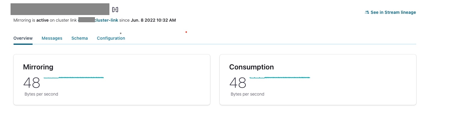
After successfully running this command, you should be able to see mirrored topic data and metrics in the Confluent Cloud console.
Bonus Round: Schema Linking
Schemas and why you need them
Kafka uses an append-only log structure to keep records of events which Kafka stores as bytes. To put objects into Kafka, producers first have to serialize the objects into bytes. When you read data from Kafka, it is the consumer’s job to deserialize the bytes back into a human-readable format. This figure from Mitch Seoymer’s book Mastering Kafka Streams and ksqlDB shows a high-level serializing and deserializing relationship in Kafka.
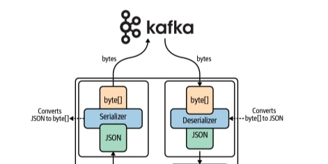
Source: “Mastering Kafka Streams and ksqlDB”
A schema can be viewed as a rule on how to convert those byte streams into readable format or vice versa. JSON, for example, is a popular data type in web programming.
When there are a lot of schemas floating around for various Kafka topics, where do you keep track of them?
A Schema Registry is where all the schemas defined by the user that Kafka is going to use are stored. In the context of Kafka, you can associate a schema with a specific Kafka topic, letting both consumers and producers know exactly what type of object should exist in that Kafka topic. Once a schema is associated with a Kafka topic, producers first have to connect to the Schema Registry and ensure that the data they’re writing to the Kafka topic is as expected. And when consumers try to get data out of a Kafka topic, they connect to Schema Registry to know how to deserialize the data.
The data that this project was mirroring from the source cluster already had a schema associated with it, but we still wanted to have the schema explicitly copied to our cluster’s Schema Registry to ensure that any client applications know how to translate the byte stream.
Sure, you could manually copy a schema from the source to the destination cluster, but what if that schema changes? Ideally, the destination cluster would be updated in real time as soon as a schema changes on the source cluster. Thankfully, Schema Linking can do just that. Schema Linking works hand-in-hand with Cluster Linking to mirror schemas from a source to a destination as they change over time.
Creating Schema Linking exporter
The process to set up Schema Linking is relatively similar to that used for Cluster Linking. First, you create a schema exporter—the object used to connect the source Schema Registry with the destination Schema Registry.
When you set up Schema Registry on your cluster, there’s a Schema Registry endpoint and you are able to create an API key and secret to use to connect to your Schema Registry. To set up Schema Linking, you need to place that information in a config.txt file.
schema.registry.url=<destination sr url>
basic.auth.credentials.source=USER_INFO
basic.auth.user.info=<destination api key>:<destination api secret>
Schema Linking is initiated from the source cluster, so Danica had to run the following command:
confluent schema-registry exporter create <exporter-name> --subjects ":*:" --config-file ~/config.txt
Once the exporter is created, from the destination cluster, you can confirm by running the following terminal command:
confluent schema-registry subject list --prefix ":*:"
Weather data
When thinking about potential factors that could affect soil moisture level, the biggest thing that comes to mind other than Danica’s watering routine is the local weather near her home in San Francisco. Many of her houseplants sit near an open window, so it’s reasonable to assume that weather might impact the plants. I decided to pull weather data from a public API, join the weather data with Danica’s ksqlDB-enriched data, and perform a simple correlation analysis.
The weather data used for this project is obtained from OpenWeatherMap. It is an open source, free-to-access, easy-to-use API with detailed instructions on its website. If you choose the free version, there is a rate limit of 60 requests per minute, which is more than sufficient for this project.
Simply go ahead and register an account and obtain your API key. The API request follows this format:
https://api.openweathermap.org/data/3.0/onecall?lat={lat}&lon={lon}&exclude={part}&appid={API key}
You also need your API key obtained from OpenWeatherMap.org, as well as the longitude and latitude of your target location for the API call.
In Python, first import the “request” and “json” modules:
import request
import json
user_api = xxx longitude = xx latitude = xx complete_api_link = "https://api.openweathermap.org/data/2.5/weather?lat="+ latitude +"&longitude=" + longitude +"&appid=" + user_api weatherData = request.get(complete_api_link) api_data = weatherData.json()
The weather data is in JSON format, and has multiple fields. In this project, we are only interested in the generic weather information:
humidity = api_data["main"]["humidity"]
pressure = api_data["main"]["pressure"]
temperature = api_data["main"]["temp"]
Now that you are familiar with how we pulled the raw data from a public API, let’s dive into how we produce messages to our Kafka topics.
Producing to Kafka with Python
You might have noticed that the data you just pulled from the api represents the weather condition at one specific point in time. What we want is a constant time stream that flows into the Kafka topics so that we can analyze the relationship between the houseplant’s soil moisture and the weather over time. We certainly cannot achieve that using one single row of stateless weather records. To set weather data in motion, we first need to create a new Kafka topic to hold the streaming weather data.
The plan is to join the weather data stream with the houseplant readings stream. Joining streams with different numbers of partitions will trigger auto repartition and create a new repartition topic in the process. To save usage and make your UI look as clean as possible, we recommend setting the number of partitions for the new topic to be the same as the topic we’re going to join with. As the readings topic is configured to have 4 partitions, set the partition count of the new topic to 4 and click launch. Once you have your topic created, the system will ask you to connect some kind of data to the topic, whether it’s a source connector connected from some database or a client application that keeps generating streaming events.
We will produce data from a client application using Python. First, prepare a Python configuration file by following the instructions on the Confluent Cloud console. After you create the topic, click configure a client and choose Python. Fill out the credentials with your API key, API secret, and bootstrap server.
Once you have your config file ready, store it in the same root directory as your Python application. Take a minute to read this script to understand how to parse arguments and read config files.
Turning JSON data into real-time streaming data
As mentioned previously, the event stream appended to the Kafka topics needs to be in bytes. The data we pulled from openWeatherAPI is in JSON format, so we need to set a schema and turn the JSON data into a byte stream following the schema we defined and then append it to the topic.
The Python JSON dumps method turns a JSON object into a string. We can use a dictionary to define a schema and pass it as a parameter to dumps, such that the byte-formatted event stream, in this case string, will be readable by Kafka when it is appended. Since we chose “humidity,” “temperature,” and “pressure” as three potential independent variables, set the schema as follows:
humidity = api_data["main"]["humidity"]
pressure = api_data["main"]["pressure"]
temperature = api_data["main"]["temp"]
Schema = {'humidity': humidity,
'pressure': pressure,
'temperature': temperature}
record_value = json.dumps(Schema)
sfproducer.produce(topic, value=record_value, on_delivery=acked)
Set data in motion
If you’ve followed along this far, you should be able to produce one record to your Kafka topic. Now it is time to create live event streams and run a program that constantly produces events. Since soil moisture and weather events are not expected to occur more frequently than every few seconds, let’s produce a weather message every 15 minutes:
while True:
       complete_api_link = xxxxx
        api_link = requests.get(complete_api_link)
        api_data = api_link.json()
        humidity = api_data["main"]["humidity"]
        pressure = api_data["main"]["pressure"]
        temperature = api_data["main"]["temp"]
        #info = {humidity, pressure, temperature, time}
        Schema = {'humidity': humidity,
                  'pressure': pressure,
                  'temperature': temperature}
        record_value = json.dumps(Schema)
        sfproducer.produce(topic, value=record_value, on_delivery=acked)
        time.sleep(15*60)
Following the template above, you have successfully built up an application that is ready to produce streaming data to Kafka topics. On your terminal, run the application, and leave it running.
python3 ./app.py -f <config file name> -t <topic name>
While your application is running in the background, you should be able to see the message being produced in the Confluent Cloud console. Since the time gap is 15 minutes between two appending messages, you need to wait a while to see messages generated in a flow.
Streaming with ksqlDB
As we have successfully built a topic that has data streams flowing in, the next step is to manipulate the data stream on ksqlDB. Being able to trim, join, and aggregate streams with SQL-like syntax on ksqlDB is one of the reasons why Kafka is so powerful and popular. ksqlDB allows you to create streams and tables that change in real time. We will mostly deal with manipulating streams in this project.
Before diving into handling ksqlDB, you need to create a ksqlDB cluster as it is separated from your main cloud cluster. Create a new ksqlDB cluster on Confluent Cloud and launch it. Once you create your cluster, let’s get started.
Creating streams
Now we have appended the weather data onto a Kafka topic that was previously created to contain the streaming events. With the weather data persisted to a Kafka topic, it can now be made available in ksqlDB. To access input data in ksqlDB, you create a stream object from an underlying Kafka topic.
But first, you must understand what your data looks like. An example event in our topic for weather events looks like this:
{
  "HUMIDITY": 94,
  "PRESSURE": 1018,
  "TEMPERATURE": 283.93
}
With that, we can create a stream as such:
CREATE STREAM SIMPLEWEATHER
  (HUMIDITY INT,
   PRESSURE INT,
   TEMPERATURE DOUBLE)
  WITH (KAFKA_TOPIC='WeatherSF',
        VALUE_FORMAT=JSON')
After the stream is created, navigate to Streams in your ksqlDB application to see your created streams. As messages are appended to the underlying Kafka topic, the stream is updated with the new events. Using the same process, we also need to create streams and tables for the topics that were mirrored via Cluster Linking. Once that is done, our cluster will look exactly like the source cluster along with an additional weather data stream to be integrated.
Joining streams
If you are familiar with SQL, you know that in order to join two tables, they must each have a field that can be referenced by the other table. In other words, two tables must have a shared field. Joining ksqlDB streams also follows the same rule.
To join the weather data stream with the houseplants reading stream, there needs to be a shared field. This is the schema of the houseplants reading stream:
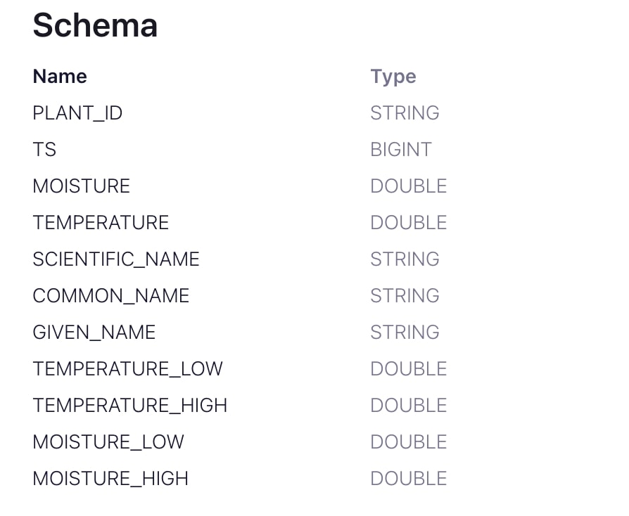
At first glance, you will not find any column that is referenceable with my simple weather stream, but our streams are still joinable! We can join two streams by timestamps. The ‘TS’ field in the houseplants stream is the timestamp when the data is read from Raspberry Pi.
But you may have noticed that our weather stream doesn’t have an explicit timestamp field. However, when an event is appended to the log in a topic, there is an implicit, hidden field called rowtime which records the record’s processing time. Knowing this, you can create another stream called weathertimed by using “create as select” semantics and explicitly selecting this hidden field. This command allows you to create a stream with a syntax similar to how streams are queried:
CREATE STREAM WEATHERTIMED
AS SELECT *, ROWTIME AS TIMESTAMP
FROM SIMPLEWEATHER EMIT CHANGES;
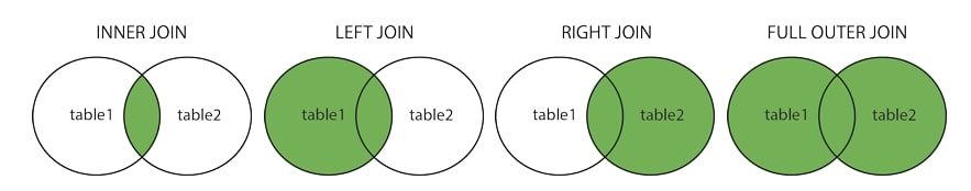
After the weathertimed stream is created, we can start joining the weather data with the plant reading data. There are four types of joins in SQL: inner, outer, left, and right. Currently on ksqlDB, joining stream with stream supports all four types of joins, but not all are supported in a stream-table or table-table joining clause. For more information, check out the documentation.
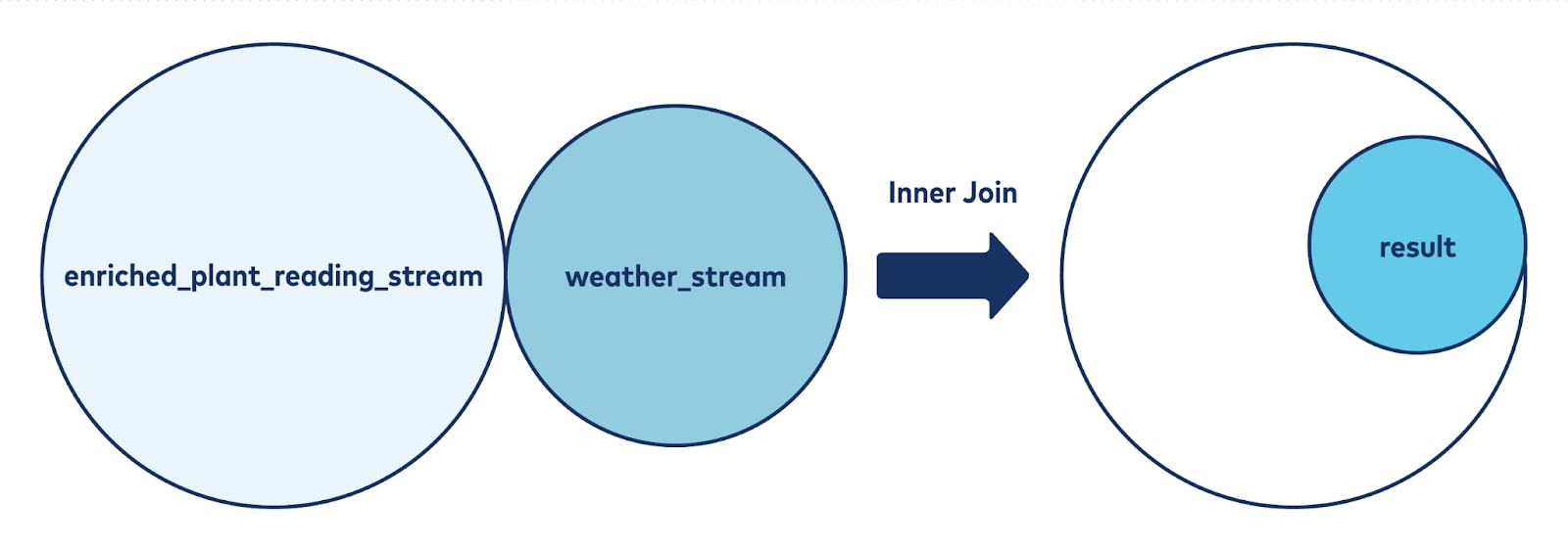
We want the joined stream to return records that have matching values in both tables, hence we should use inner join.
With a record appended every few seconds, the houseplant stream has a much larger sample size, while the weather data is produced every 15 minutes. Conducting an inner join ensures that after joining, we will still have a relatively big sample size for training models because almost all the records in the weather stream are included in the join. Joining data should look like this:
Let’s create another stream to store the result of this inner join:
CREATE STREAM WEATHERPLANTENRICHED AS
SELECT
    w.TIME,
    w.ROWTIME/1000 as TS,
    w.Humidity,
    w.PRESSURE,
    w.TEMPERATURE,
    h.*
FROM WEATHERTIMED  w
INNER JOIN
HOUSEPLANT_READINGS_ENRICHED h
WITHIN 7 DAYS on
w.ROWTIME/1000 = h.TS
EMIT CHANGES;
You might have noticed that the timestamp from the weathertimed stream was divided by 1000. This is because the default timestamp unit is in milliseconds whereas the timestamp unit in the houseplant readings topic is in seconds. In order to join two streams, we need them to be in the same unit.
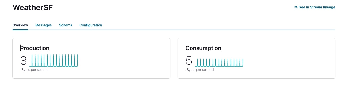
Every time a new stream is created in Confluent Cloud, there will be a new corresponding topic automatically created at the same time. We will use those topics for consuming the integrated data.
ksqlDB on Confluent Cloud has a feature that comes in handy whenever you have multiple streams created, allowing you to easily visualize the relationships between them. Click into your ksqlDB cluster to see a flow tab; click into that, there is a display of the Stream Lineage (part of Confluent Cloud’s Stream Governance feature set) in this cluster. This is extremely useful when you have streams that you want to delete, or when you want to figure out relationships between two streams.
Consuming Kafka data with Python
Now the data is well structured on Kafka topics thanks to Cluster Linking and ksqlDB. The next step is to read the final enriched record so that you can do some analysis with the enriched streaming data. The action of reading data is called consuming, and it is done by a Kafka object called consumer.
Configuration
Similar to producer, the consumer instance also needs a .config file. Luckily, you can start by reading the same file used to configure for the producer. From there, you need to manually alter a few configuration values.
config_file = "python.config"
conf = ccloud_lib.read_ccloud_config(config_file)
consumer_conf = ccloud_lib.pop_schema_registry_params_from_config(conf)
First, you need to specify a group ID for the consumer you created. This helps to store consumer offsets, allowing your consumer to keep track of where they left off in consuming data from the topic.
consumer_conf[‘group_id’] = ‘<your choice of id name>’
But when you first start a consumer group instance, there is no consumer offset, so you need to tell the consumer where to start reading from the topic. You can read from the latest offset to obtain the newest messages, or the earliest offset to obtain data from the beginning of the topic. In this case, we want all of the data, so we’ll use earliest.
consumer_conf['auto.offset.reset'] = 'earliest'
Now that the configuration is set up, you create your consumer instance using the subscribe function to subscribe to the topic backing the ksqlDB stream created above:
weatherConsumer = Consumer(consumer_conf)
enriched_consumer = Consumer(consumer_conf)
enriched_consumer.subscribe(["pksqlc-pj1gyWEATHER_PLANT_ENRICHED"])
At this point, the consumer is ready to read data from the subscribed topic!
Consumption loop
The loop is very similar to the loop you had with producer loop, except you need to deserialize the stream data to JSON format. Luckily, the JSON library has a very useful function to do it:
try:
    while True:
        msg = enriched_consumer.poll(1.0)
        if msg is None:
            print("Waiting for message or event/error in poll()")
            continue
        elif msg.error():
            print('error: {}'.format(msg.error()))
            continue
        else:
            record_key = msg.key()
            record_value = msg.value()
            data = json.loads(record_value)
            curr_value_list = list(data.values())
            df0.loc[len(df0)] = curr_value_list
Data analysis
The next step is to convert the streaming data to batch data so that you can easily conduct analysis.
Note that since different plants might be placed at different locations and have different soil properties, you need to do data analysis for each plant. Both the houseplant readings topic and the weather topic have a retention period of seven days, meaning that all events written to Kafka topics prior to seven days ago are expired. Because of this, there are at most 4*24*7 = 672 records of enriched data stored in the topic for each plant since weather events occur every 15 minutes. You will have to train a model for each plant, but the training process is repetitive, and you can easily repeat the training process in a for loop if you ever want to scale up the project with a larger number of plants. Kafka is a great tool for doing streaming analytics which is faster when dealing with large volumes of streaming data. However, for simplicity of the project, the following data analysis was conducted in batch.
Import Pandas DataFrame first and create an empty skeleton of a Pandas table, set the field name to what you had for each of the records consumed by your consumer.
df0 = pd.DataFrame({'WEATHER_TIME': pd.Series(dtype= 'str'),
                    'WEATHER_TIMESTAMP': pd.Series(dtype='int'),
                    'WEATHER_HUMIDITY': pd.Series(dtype='int'),
                    "WEATHER_PRESSURE": pd.Series(dtype='int'),
                    "SF_TEMPERATURE": pd.Series(dtype='float'),
                    "PLANT_ID": pd.Series(dtype='str'),
                    "PLANT_MOISTURE": pd.Series(dtype='float'),
                    "PLANT_TERMPERATURE": pd.Series(dtype='float'),
                    "PLANT_SCIENTIFIC_NAME": pd.Series(dtype='str'),
                    "PLANT_COMMON_NAME": pd.Series(dtype='str'),
                    "PLANT_GIVEN_NAME": pd.Series(dtype='str'),
                    "PLANT_TEMPERATURE_LOW": pd.Series(dtype='float'),
                    "PLANT_TEMPERATURE_HIGH": pd.Series(dtype='float'),
                    "PLANT_MOISTURE_LOW": pd.Series(dtype='float'),
                    "PLANT_MOISTURE_HIGH": pd.Series(dtype='float'),
                    })
For every loop, you will consume a message from your topic and deserialize it to JSON format and append it to a Pandas data frame:
Data = json.loads(record_value)
            curr_value_list = list(data.values())
            df0.loc[len(df0)] = curr_value_list
Finally, save the data frame to a csv file for better readability, and close the consumer instance:
finally:
    df0 = df0.sort_values('WEATHER_TIMESTAMP', ascending=True)
    df0.to_csv(<"tablename">)
    display(df0)
    enriched_consumer.close()
A regression analysis is used to determine if there’s a significant correlation between the moisture in the plants and the weather data. Print the correlation between soil moisture and each of the variables first:
correlation0M = numpy.corrcoef(plant0['PLANT_MOISTURE'], plant0['WEATHER_HUMIDITY'])[0, 1]
correlation0T = numpy.corrcoef(plant0['PLANT_MOISTURE'], plant0['SF_TEMPERATURE'])[0, 1]
correlation0P = numpy.corrcoef(plant0['PLANT_MOISTURE'], plant0['WEATHER_PRESSURE'])[0, 1]
print([correlation0P, correlation0T, correlation0M]) [0.2676099024539299, -0.19387139547880258, -0.11382208880140181]
The most correlated field is moisture, and it’s only 26.76%, whereas the rest of the variables are barely correlated with the moisture level. Run a simple regression model with sklearn to train a prediction model:
X_train, X_test, y_train, y_test = train_test_split(plant0[['WEATHER_HUMIDITY']], plant0['PLANT_MOISTURE'],
                                                    test_size=0.2, random_state=1)
#fit regression
plant0_reg = linear_model.LinearRegression()
plant0_reg.fit(X_train, y_train)
plant_moisture_pred = plant0_reg.predict(X_test)
print("Mean squared error: %.2f" % mean_squared_error(y_test, plant_moisture_pred))
Mean squared error: 751.99
To be more statistically prudent, import the statsmodels package to do an Anova analysis. At the top of the script:
from statsmodels.formula.api import ols
from statsmodels.stats.anova import anova_lm
Fit humidity data and soil moisture variable in another data frame and construct a linear regression model:data = pd.DataFrame({'x': plant0['WEATHER_HUMIDITY'], 'y': plant0['PLANT_MOISTURE']}) model = ols("y ~ x", data).fit() anova_results = anova_lm(model) print('\nANOVA results') print(anova_results)
ANOVA results df sum_sq mean_sq F PR(>F) x 1.0 2741.044555 2741.044555 3.596391 0.058957 Residual 274.0 208833.294241 762.165307 NaN NaN
The p value in this case is slightly over 5%, which implies that the model is not statistically significant under the 5% significance level. While we found no correlation with our current plant sample and weather conditions, we could repeat the process with more plants, under different conditions and in different locations (such as outdoors).
Now, you’ve successfully learned how to build a data pipeline with Apache Kafka on the Confluent Cloud!
Try it yourself!
If you followed the tutorial so far, congratulations! You should now have a clear picture of what Kafka is, how to share data quickly and reliably between clusters with minimal data loss thanks to Cluster Linking, and how to build a complete data pipeline with Kafka on Confluent Cloud. From there, you saw how to utilize ksqlDB to join data streams together and create a consumer to batch the data for analysis.
This is only the tip of the iceberg of what is possible when you run Apache Kafka on Confluent Cloud. Git it a try by building a data pipeline with Confluent and manipulate the data stream with ksqlDB on your own. Hands-on experience is the best way to make sure you understand the technology. Check out the original or extension project repositories to get started.
If you’d like to keep learning more about how to use Apache Kafka, check out the library of free courses on Confluent Developer!
Did you like this blog post? Share it now
Subscribe to the Confluent blog


Confluent and Amazon EventBridge for Broad Event Distribution
Learn how to stream real-time data from Confluent to AWS EventBridge. Set up the connector, explore use cases, and build scalable event-driven apps.


New With Confluent Platform 8.0: Stream Securely, Monitor Easily, and Scale Endlessly
This blog announces the general availability (GA) of Confluent Platform 8.0 and its latest key features: Client-side field level encryption (GA), ZooKeeper-free Kafka, management for Flink with Control Center, and more.