[Webinar] How to Implement Data Contracts: A Shift Left to First-Class Data Products | Register Now
Detecting Patterns of Behaviour in Streaming Maritime AIS Data with Confluent
This is part two in a blog series on streaming a feed of AIS maritime data into Apache Kafka® using Confluent and how to apply it for a variety of purposes. The first blog post Streaming ETL and Analytics on Confluent with Maritime AIS Data looked at building out streaming analytics on the data using Confluent. The data begins its life as a binary stream:
$ nc 153.44.253.27 5631
\s:2573485,c:1614772291*0C\!BSVDM,1,1,,A,13maq;7000151TNWKWIA3r<v00SI,0*01
\s:2573250,c:1614772291*02\!BSVDO,1,1,,B,402M3hQvDickN0PTuPRwwH7000S:,0*37
!BSVDM,1,1,,A,13o;a20P@K0LIqRSilCa?W4t0<2<,0*19
\s:2573450,c:1614772291*04\!BSVDM,1,1,,B,13m<?c00000tBT`VuBT1anRt00Rs,0*0D
\s:2573145,c:1614772291*05\!BSVDM,1,1,,B,13m91<001IPPnJlQ9HVJppo00<0;,0*33
The stream is ingested into Kafka on Confluent Cloud:
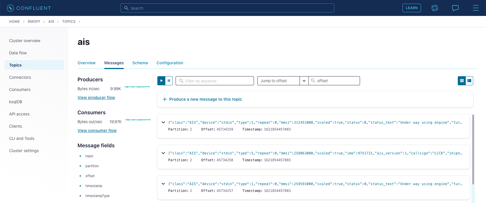
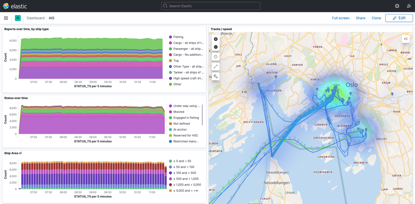
Using stream processing, it’s then available for analytics and visualisation:
The inspiration for this series came from a question on Stack Overflow that piqued my curiosity. In an offline discussion with the author, he revealed that he was investigating the behaviour of ships to identify potential illegal fishing activities. In this particular case, it was transshipping—the uses of which can be perfectly legal, but not always. According to Global Fishing Watch:
Large vessels with refrigerated holds collect catch from multiple fishing boats and carry it back to port. By enabling fishing vessels to remain on the fishing grounds, transshipment reduces fuel costs and ensures catch is delivered to port more quickly. It also leaves the door open for mixing illegal catch with legitimate catch, drug smuggling, forced labor and human rights abuses aboard fishing vessels that remain at sea for months or years at a time.
Global Fishing Watch has done a lot of work in identifying suspected illegal fishing and published detailed reports on their findings and techniques used. Their approach is to take a historical look at the data and retrospectively identify patterns. This blog post is designed to show how stream processing can be used to look for these patterns as they occur.
The specs used are based on those described in Identifying Global Patterns of Transshipment Behavior:
Encounters were identified from AIS data as locations where a fishing vessel and a transshipment vessel were continuously within 500 m for at least 2 h and traveling at < 2 knots, while at least 10 km from a coastal anchorage.
In my example, I built the first part of this (“within 500 m for at least 2 h and traveling at < 2 knots”) but not the second (“at least 10 km from a coastal anchorage”), and thus as you will see later on, there are plenty of false positives identified. And, it bears repeating, transshipping is not itself illegal—so no comment whatsoever is made about the behaviour of any ships identified here.
Let’s break the problem down into pieces.
Identifying fishing and transshipment vessels
First up, we need to identify ships that are fishing, and those that are transshipment vessels, or reefers (refrigerated cargos), as they are often known. Similar to the first blog post on streaming ETL, the information about ships in general is collected from AIS, and this data is streamed into a Kafka topic. From here, we model the stream of events as a table, against which we can then query.
Global Fishing Watch used machine learning to create a list of fishing vessels based on the reported ship type in the AIS data as well as other attributes. In my initial proof of concept, I just used the AIS attribute alone, but as we see shortly, incorporating the list here would be easily done.
For reefers, there are two sources of data, both also from Global Fishing Watch.
- A list of carriers, from which a list of unique MMSIs and ship name was extracted to Reefers.csv
- A list of transshipment vessels, written to transshipment-vessels-v20170717.csv
This is where the fun bit of data engineering comes in, because the reality is that datasets are frequently imperfect, or in different formats, or just need wrangling for other reasons. Here I wanted to see what the overlap was between the two sets of data that I had for reefers. I could have used various tools but had comm to hand. Each file needed a bit of pre-processing using process substitution to fix CRLF line breaks and extract just the mmsi field:
- MMSI in both files:
$ comm -12 <(tr -d '\r' < Reefer.csv |awk -F";" ' { print $2}'|sort) <(tr -d '\r' < transshipment-vessels-v20170717.csv|awk -F"," '{print $1}'|sort) | wc -l 501 - MMSI only in Reefers.csv:
$ comm -23 <(tr -d '\r' < Reefer.csv |awk -F";" ' { print $2}'|sort) <(tr -d '\r' < transshipment-vessels-v20170717.csv|awk -F"," '{print $1}'|sort) | wc -l 326 - MMSI only in transshipment-vessels-v20170717.csv:
$ comm -13 <(tr -d '\r' < Reefer.csv |awk -F";" ' { print $2}'|sort) <(tr -d '\r' < transshipment-vessels-v20170717.csv|awk -F"," '{print $1}'|sort) | wc -l
     624
Because there were clearly plenty of reefers in each file that weren’t in the other, I decided to load both into Kafka. I did this using kafkacat and a technique to set the key column correctly at ingest:
$ ccloud kafka topic create reefers
$ tr -d '\r' < Reefer.csv | \
  awk -F";" ' { print $2 "\x1c" $1 } '| \
  docker run --rm --interactive edenhill/kafkacat:1.6.0 \
  kafkacat -X security.protocol=SASL_SSL -X sasl.mechanisms=PLAIN \
           -X ssl.ca.location=./etc/ssl/cert.pem -X api.version.request=true \
           -b $CCLOUD_BROKER:9092 \
           -X sasl.username="$CCLOUD_API_KEY" \
           -X sasl.password="$CCLOUD_API_SECRET" \
           -t reefers -K$'\x1c' -P

$ ccloud kafka topic create transshipment-vessels
$ tr -d '\r' < transshipment-vessels-v20170717.csv | \
  sed  "s/,/$(printf '\x1c')/" | \
  docker run --rm --interactive edenhill/kafkacat:1.6.0 \
  kafkacat -X security.protocol=SASL_SSL -X sasl.mechanisms=PLAIN \
           -X ssl.ca.location=./etc/ssl/cert.pem -X api.version.request=true \
           -b $CCLOUD_BROKER:9092 \
           -X sasl.username="$CCLOUD_API_KEY" \
           -X sasl.password="$CCLOUD_API_SECRET" \
           -t transshipment-vessels -K$'\x1c' -P
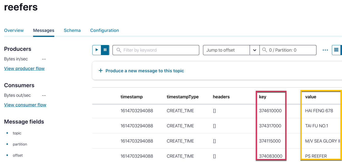
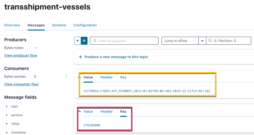
With the data now in topics in Confluent Cloud, I could inspect it to check that the key had been set correctly on both (different options in the topic viewer enable inspection of the data to suit its contents best).
The next step was to define a ksqlDB table on each of the Kafka topics. Because the data is delimited, I had to declare the full schema. Note also the PRIMARY KEY specification on each, which denotes that that field comes from the key of the Kafka message (rather than the value).
CREATE TABLE reefers_raw (mmsi         VARCHAR PRIMARY KEY,
                          shipname_raw VARCHAR)
  WITH (KAFKA_TOPIC='reefers',
        FORMAT     ='DELIMITED');

CREATE TABLE transshipment_vessels_raw (mmsi            VARCHAR PRIMARY KEY,
                                        shipname        VARCHAR,
                                        callsign        VARCHAR,
                                        flag            VARCHAR,
                                        imo             VARCHAR,
                                        first_timestamp VARCHAR,
                                        last_timestamp  VARCHAR)
  WITH (KAFKA_TOPIC='transshipment-vessels',
        FORMAT     ='DELIMITED');
With the tables created, the next step is to integrate the data into the existing pipeline (as it’s the same logical entities). Using a LEFT OUTER JOIN, I added in two new attribute fields to the existing SHIP_INFO table. Note that whilst evolvable queries (CREATE OR REPLACE) have been recently added to ksqlDB, the change I was making to the table wasn’t supported so I had to rebuild it. But since Kafka stores data, it was easy enough to just rebuild this table from the original data stream (AIS_MSG_TYPE_5), by setting 'auto.offset.reset' = 'earliest' so that ksqlDB reconsumes all of the data from the beginning of the topic.
DROP TABLE SHIP_INFO;

SET 'auto.offset.reset' = 'earliest';

CREATE TABLE SHIP_INFO AS
  SELECT A.MMSI                                                       AS MMSI,
         MAX(ROWTIME)                                                 AS LAST_INFO_PING_TS,
         LATEST_BY_OFFSET(SHIPNAME)                                   AS SHIPNAME,
         LATEST_BY_OFFSET(DRAUGHT)                                    AS DRAUGHT,
         LATEST_BY_OFFSET(DESTINATION)                                AS DESTINATION
         LATEST_BY_OFFSET(CASE WHEN R.MMSI IS NULL THEN 0 ELSE 1 END) AS IS_REEFER,
         LATEST_BY_OFFSET(CASE WHEN T.MMSI IS NULL THEN 0 ELSE 1 END) AS IS_TRANSSHIPPER
    FROM AIS_MSG_TYPE_5 A
        LEFT JOIN REEFERS_RAW R ON A.MMSI=R.MMSI
        LEFT JOIN TRANSSHIPMENT_VESSELS_RAW T ON A.MMSI=T.MMSI
GROUP BY A.MMSI ;
Now we can use the updated table to look up information about a ship by its MMSI, as well as analyse the data that we have. Bear in mind that the row counts shown from comm above are for the entire file, whilst the SHIP_INFO table is driven by AIS type 5 messages received around Norway—so we can only expect to see ships identified with the reefer/transshipper flags that are sailing in those waters and have reported a type 5 message in the time sample.
ksql> SELECT CASE
              WHEN IS_REEFER =0 AND IS_TRANSSHIPPER = 0 THEN 'Neither'
              WHEN IS_REEFER =1 AND IS_TRANSSHIPPER = 0 THEN 'Reefer.csv only'
              WHEN IS_REEFER =0 AND IS_TRANSSHIPPER = 1 THEN 'transshiper.csv only'
              WHEN IS_REEFER =1 AND IS_TRANSSHIPPER = 1 THEN 'Both'
            END AS LABEL,
            COUNT(*) AS CT
        FROM SHIP_INFO
        GROUP BY CASE
              WHEN IS_REEFER =0 AND IS_TRANSSHIPPER = 0 THEN 'Neither'
              WHEN IS_REEFER =1 AND IS_TRANSSHIPPER = 0 THEN 'Reefer.csv only'
              WHEN IS_REEFER =0 AND IS_TRANSSHIPPER = 1 THEN 'transshiper.csv only'
              WHEN IS_REEFER =1 AND IS_TRANSSHIPPER = 1 THEN 'Both'
            END
        EMIT CHANGES;

+---------------------+-----+
|LABEL                |CT   |
+---------------------+-----+
|transshiper.csv only |6    |
|Reefer.csv only      |8    |
|Both                 |6    |
|Neither              |3223 |
…
Identifying vessels that are close to each other for a period of time
Having built a table that enables us to characterise ships as fishing vessels or reefers, we now come to the crux of the requirement:
…where a fishing vessel and a transshipment vessel were continuously within 500 m for at least 2 h and travelling at < 2 knots
I solved this using two hops:
- Create a stream of ships close to each other at any time and travelling at a slow speed
…where a fishing vessel and a transshipment vessel were continuously within 500 m … and travelling at < 2 knots
- Create a windowed aggregate on this stream to identify those that had been close for longer than two hours
for at least 2 h
Stream-stream joins in ksqlDB
When we built the streaming ETL pipeline above, we used a stream-table join to enrich a stream of events with supplemental information. Now we’re going to use a stream-stream join. The two streams are both going to be from the AIS data of ship position reports, but one stream will only be fishing vessels, and the other reefers. We can use the GEO_DISTANCE function to determine the distance between them (based on the great-circle distance) and use this as a predicate in the resulting stream.
When doing a stream-stream join, ksqlDB requires two unique source streams, for various reasons. This is the case even if the underlying data is the same, so what we do here is a bit of a kludgy workaround. First up, we rebuild SHIP_STATUS_REPORTS to include a literal value in a field called DUMMY (you’ll see why in a moment):
DROP STREAM SHIP_STATUS_REPORTS;

SET 'auto.offset.reset' = 'earliest';

CREATE STREAM SHIP_STATUS_REPORTS WITH (KAFKA_TOPIC='SHIP_STATUS_REPORTS_V00') AS
SELECT STATUS_REPORT.ROWTIME AS STATUS_TS, STATUS_REPORT.*,  SHIP_INFO.*,
       1 AS DUMMY
FROM  AIS_MSG_TYPE_1_2_3 STATUS_REPORT
      LEFT JOIN SHIP_INFO SHIP_INFO
        ON STATUS_REPORT.MMSI = SHIP_INFO.MMSI;
Then we clone this stream into a new one, with a predicate to include only events that come from what we think may be a reefer (i.e., a ship whose MMSI appears on one or both of the Reefer.csv/transshipper.csv):
CREATE STREAM REEFER_MOVEMENTS AS
  SELECT *
    FROM SHIP_STATUS_REPORTS
   WHERE (SHIP_INFO_IS_TRANSSHIPPER=1
       OR SHIP_INFO_IS_REEFER=1);
Now we build our stream-stream join, between SHIP_STATUS_REPORTS (with a predicate to include only fishing vessels) and REEFER_MOVEMENTS.
CREATE STREAM REEFERS_AND_VESSELS_WITHIN_500M
  WITH (KAFKA_TOPIC='REEFERS_AND_VESSELS_WITHIN_500M_V00') AS
SELECT    V.STATUS_REPORT_MMSI   AS FISHING_VESSEL_MMSI,
          R.STATUS_REPORT_MMSI   AS REEFER_MMSI,
          V.SHIP_LOCATION        AS FISHING_VESSEL_LOCATION,
          R.SHIP_LOCATION        AS REEFER_LOCATION,
          GEO_DISTANCE(V.STATUS_REPORT_LAT, V.STATUS_REPORT_LON, R.STATUS_REPORT_LAT, R.STATUS_REPORT_LON, 'KM') AS DISTANCE_KM,
          CASE
            WHEN GEO_DISTANCE(V.STATUS_REPORT_LAT, V.STATUS_REPORT_LON, R.STATUS_REPORT_LAT, R.STATUS_REPORT_LON, 'KM') < 0.5
                 AND  (    R.STATUS_REPORT_SPEED <2
                       AND V.STATUS_REPORT_SPEED < 2) THEN 1
                 ELSE 0
             END AS IN_RANGE_AND_SPEED
FROM      SHIP_STATUS_REPORTS V
          INNER JOIN REEFER_MOVEMENTS R
            WITHIN 1 MINUTE
            ON     R.DUMMY = V.DUMMY
WHERE     V.SHIP_INFO_SHIPTYPE_TEXT  = 'Fishing'
AND       V.STATUS_REPORT_MMSI      != R.STATUS_REPORT_MMSI
AND       GEO_DISTANCE(V.STATUS_REPORT_LAT, V.STATUS_REPORT_LON, R.STATUS_REPORT_LAT, R.STATUS_REPORT_LON, 'KM') < 1
PARTITION BY V.STATUS_REPORT_MMSI;
This stream includes an IN_RANGE_AND_SPEED flag, which we’ll use in the next step, and hardcodes the predicates of the pattern that we’re looking for (distance is less than 0.5 km, both ships moving at less than two knots). The resulting stream only includes ships that are within 1 km of each other (regardless of speed). Why 1 km? Because when I was testing, I wanted to make sure that it worked, so I included values over 500 m too 🙂
+--------------------+------------+-------------------------------+------------------------------+----------------------+-------------------+
|FISHING_VESSEL_MMSI |REEFER_MMSI |FISHING_VESSEL_LOCATION        |REEFER_LOCATION               |DISTANCE_KM           |IN_RANGE_AND_SPEED |
+--------------------+------------+-------------------------------+------------------------------+----------------------+-------------------+
|258036000           |257430000   |{lat=62.324023, lon=5.66427}   |{lat=62.321373, lon=5.653208} |0.642853083812366     |0                  |
|273844800           |273440860   |{lat=69.728918, lon=30.034538} |{lat=69.72819, lon=30.03179}  |0.1332701769571591    |1                  |
|273433220           |273440860   |{lat=69.72493, lon=30.023542}  |{lat=69.72819, lon=30.03179}  |0.4820709202116538    |1                  |
|273433400           |273440860   |{lat=69.727357, lon=30.03141}  |{lat=69.72819, lon=30.03179}  |0.09377524348557457   |1                  |
|257810500           |258211000   |{lat=62.55565, lon=6.26555}    |{lat=62.548723, lon=6.276892} |0.9649975921607864    |0                  |
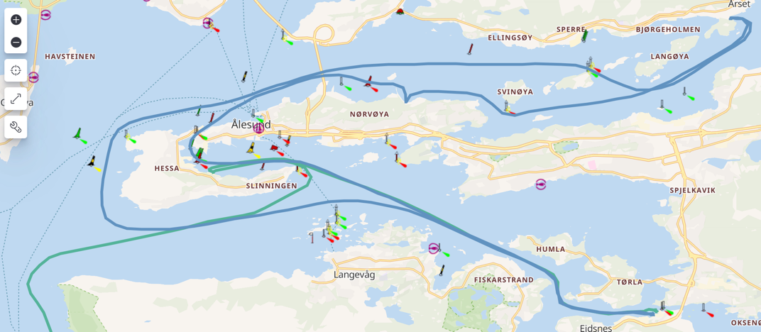
With Kibana, we can use this stream to plot on the map where these types of ships are close to each other, regardless of how long or at what speed. Here we can see two ships close by for part of their journey:
Session windows in ksqlDB
With this stream of events, we can now look at which ships match the requirement in terms of the duration of their proximity and speed. I used a windowed aggregation here with a session window to group the aggregates. You can learn more about windowed aggregates in ksqlDB in the documentation, but whereas a tumbling window has a fixed duration, a session window varies depending on the continuing arrival of events within a given timeout.
SELECT FISHING_VESSEL_MMSI,
       REEFER_MMSI,
       TIMESTAMPTOSTRING(MIN(ROWTIME),'HH:mm:ss','Europe/Oslo') AS FIRST_TIME,
       TIMESTAMPTOSTRING(MAX(ROWTIME),'HH:mm:ss','Europe/Oslo') AS LAST_TIME,
       (MAX(ROWTIME) - MIN(ROWTIME)) / 1000                     AS DIFF_SEC,
       MAX(DISTANCE_KM) AS FURTHEST_DISTANCE,
       COUNT(*) AS EVENT_CT
FROM   REEFERS_AND_VESSELS_WITHIN_1KM WINDOW SESSION (10 MINUTES)
WHERE  IN_RANGE_AND_SPEED=1
GROUP BY FISHING_VESSEL_MMSI, REEFER_MMSI
EMIT CHANGES;
+--------------------+------------+-----------+----------+---------+-------------------+---------+
|FISHING_VESSEL_MMSI |REEFER_MMSI |FIRST_TIME |LAST_TIME |DIFF_SEC |FURTHEST_DISTANCE  |EVENT_CT |
+--------------------+------------+-----------+----------+---------+-------------------+---------+
|273433220           |273440860   |11:57:14   |12:33:13  |2159     |0.4846046047267392 |13       |
|258036000           |257430000   |13:01:07   |13:04:54  |227      |0.4997634317289095 |4        |
|257888000           |258211000   |11:57:54   |13:33:45  |5751     |0.3039245344432804 |58       |
The 10 MINUTES session window timeout is unrelated to the two-hour time period that we’re going to build into a predicate. The session window timeout means that if two ships are close to one another and within speed parameters, but there is no event received from both within 10 minutes, then the session window “closes.” If events are subsequently received, that counts as a new window. The window is important because that gives us the duration of the window (DIFF_SEC) against which we can build a predicate. If you want to allow for greater “blackouts” in events, you can increase the timeout on the session window—but bear in mind that it could be that events were received from both ships but one or the other predicate (speed/distance) wasn’t matched. In this scenario, you’d end up with logically invalid results.
Using this session windowing logic, combined with a HAVING predicate, we can now build out a table of fishing vessels and reefers that are close together, at slow speed, and for more than two hours (7,200 seconds):
CREATE TABLE REEFERS_AND_VESSELS_CLOSE_FOR_GT_2HR
  WITH (KAFKA_TOPIC='REEFERS_AND_VESSELS_CLOSE_FOR_GT_2HR_V00') AS
SELECT   FISHING_VESSEL_MMSI,
         REEFER_MMSI,
         STRUCT("lat":=LATEST_BY_OFFSET(FISHING_VESSEL_LAT),"lon":=LATEST_BY_OFFSET(FISHING_VESSEL_LON)) AS LATEST_FISHING_VESSEL_LOCATION,
         STRUCT("lat":=LATEST_BY_OFFSET(REEFER_LAT),        "lon":=LATEST_BY_OFFSET(REEFER_LON))         AS LATEST_REEFER_LOCATION,
         MIN(DISTANCE_KM)                                                                                AS CLOSEST_DISTANCE_KM,
         MAX(DISTANCE_KM)                                                                                AS FURTHEST_DISTANCE_KM,
         MIN(FISHING_VESSEL_TS)                                                                          AS FIRST_TS,
         MAX(FISHING_VESSEL_TS)                                                                          AS LAST_TS,
         (MAX(FISHING_VESSEL_TS) - MIN(FISHING_VESSEL_TS)) / 1000                                        AS DIFF_SEC
FROM     REEFERS_AND_VESSELS_WITHIN_1KM WINDOW SESSION (10 MINUTES)
WHERE    IN_RANGE_AND_SPEED = 1
GROUP BY FISHING_VESSEL_MMSI,
         REEFER_MMSI
HAVING   (MAX(ROWTIME) - MIN(ROWTIME)) / 1000 > 7200;
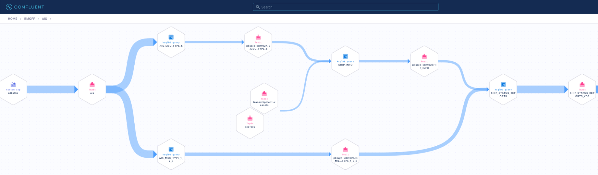
That’s a fair bit of processing we’ve done. Here’s a nice breakdown of it from the Data Lineage view in Confluent Cloud:
Visualising the results
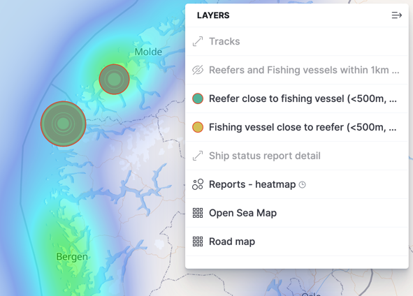
Tables in ksqlDB are backed by Kafka topics, which means that we can stream the continually updated table over to Elasticsearch (using the managed connector as in part 1 of this series), from where it can be plotted in Kibana alongside the existing map view:
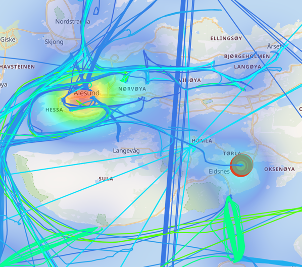
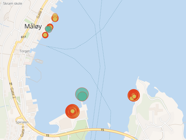
Zooming in, we can see that it’s in the Ålesund municipality:
And going right down to the detail—the reason the ships are close together for this period of time is…they’re in port!
We can see the same behaviour repeating for other matches of the pattern:
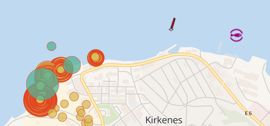
Hence the necessity of the additional step in the original requirements on which this idea was based:
at least 10 km from a coastal anchorage
But that is a project for another day. It’d be entirely doable in ksqlDB—load a Kafka topic with a list of lat/long of coastal anchorages, build a ksqlDB table on that, and do a negated join to the stream of vessels identified as close to each other.
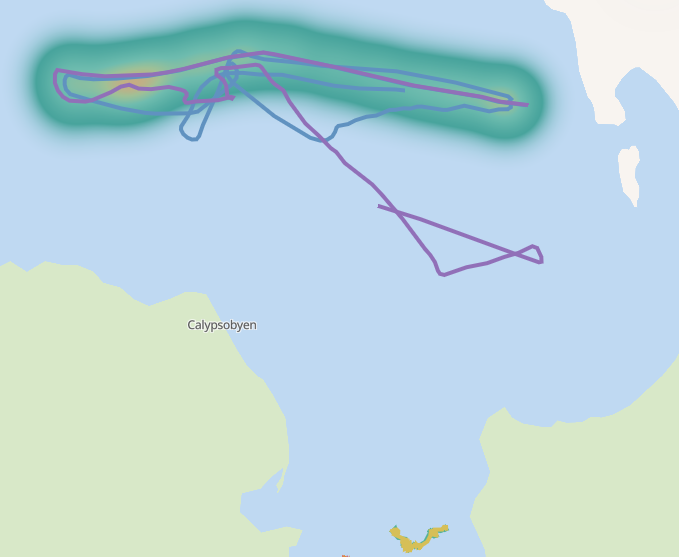
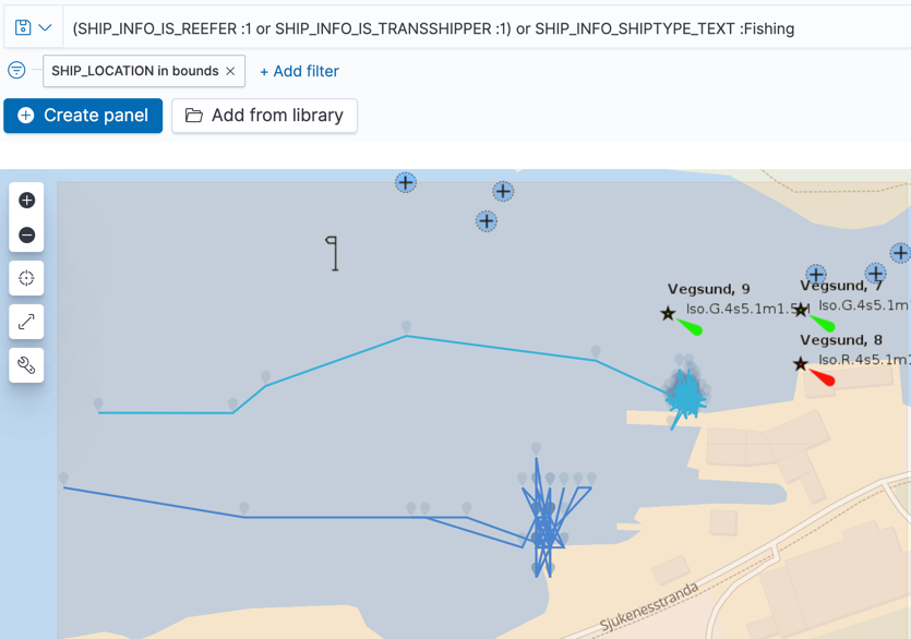
You can use the map visualisation even further to look at the route that the two vessels took—the fishing vessel (blue) looping around the local area whilst the transhipper (green) continues out and beyond.
What else can we do with the pattern matches (once we make them a tad more precise)? Visualisation on an interactive map is pretty powerful, but let’s remember this is data on a Kafka topic, so we can do other things as well:
- Write it to a database, from where reporting could be driven
- Build a microservice that subscribes to the topic and drive real-time alerts to prompt action on suspicious behaviour
Summary
The most interesting examples of technology in action are where it fulfills a real requirement. Tools can be fun for the sake of tools, but the AIS data has shown just how useful streams of events can be and what’s possible to build with a bit of SQL and some managed cloud services like Confluent Cloud.
You can try Confluent Cloud using code RMOFF200 for $200 off your bill.
If you’d rather run this on premises, you can do that using the Docker Compose file and instructions in the GitHub repo.
Acknowledgments
My huge thanks to Lars Roar Uggerud Dugstad for prompting my curiosity with his question on StackOverflow, and for all his help in scratching the figurative itch that it prompted!
AIS data distributed by the Norwegian Coastal Administration under Norwegian licence for Open Government data (NLOD).
Datasets distributed by Global Fishing Watch under Creative Commons Attribution-ShareAlike 4.0 International license.
Did you like this blog post? Share it now
Subscribe to the Confluent blog


3 Strategies for Achieving Data Efficiency in Modern Organizations
The efficient management of exponentially growing data is achieved with a multipronged approach based around left-shifted (early-in-the-pipeline) governance and stream processing.


Chopped: AI Edition - Building a Meal Planner
Dinnertime with picky toddlers is chaos, so I built an AI-powered meal planner using event-driven multi-agent systems. With Kafka, Flink, and LangChain, agents handle meal planning, syncing preferences, and optimizing grocery lists. This architecture isn’t just for food, it can tackle any workflow.