New in Confluent Cloud: Making Data & Pipelines Accessible for AI-Ready Streaming | Learn More
Preventing Fraud and Fighting Account Takeovers with Kafka Streams
Many companies have recently started to take cybersecurity and data protection even more seriously, particularly driven by the recent General Data Protection Regulation (GDPR) legislation. They are increasing their investment not only to avoid fines—4% of annual income would hurt even the biggest players—but also to avoid damaged reputations and financial loss due to hackers. According to research conducted by Javelin Strategy & Research, every two seconds, another American becomes a victim of online identity fraud. Building a fraud prevention system that detects compromised accounts, and malicious user behavior is the main goal of this blog post.
For the purposes of this post, let’s assume that we just want to analyze website login attempts by using Kafka Streams’ real-time stream processing technology. These attempts will flow into the system as events, and our risk detection platform will consume the events and seek to detect any of the following situations:
- Login attempts using a new device for a given user
- Login attempts from a new location for a given user
- Login attempts from botnet agents
- Brute-force attacks
There are many values we could gather from a website login attempt, but in this article, we will focus on the device used in the attempt, the location, and the device’s IP address.
Real-time fraud prevention using Apache Kafka®
As our requirements stand, we need to perform four different types of analysis. Each new login event will trigger an analysis. An event is a statement of a fact: something that happened in the system. A recorded sequence of these facts is an event stream.
As a prerequisite for stream processing, we need a strong foundation—a reliable, scalable, and fault-tolerant event streaming platform that stores our input events and process results. Apache Kafka is an industry standard that serves exactly this purpose. Its core abstraction for a stream of records of a given type is the topic, and each record in a Kafka topic consists of a key, a value, and a timestamp.
We can start out building processing applications using Kafka’s consumer and producer APIs, but at some point, as the processing logic becomes more and more sophisticated, we’ll discover a lot of additional technical work that we need to do. Moreover, as we start to identify some common patterns, we’ll want to use a higher level of abstraction. Luckily, we do not need to build our own abstractions: the Kafka Streams API comes to the rescue.
Kafka Streams is a library that can be used with any application built on a JVM stack; it does not require a separate processing cluster. Such an application, also known as a stream processor, can be deployed on any platform of the user’s choice, as Kafka Streams has no opinions about deployment platforms. The library provides a clearly defined DSL for processing operations, including stateless and stateful operators as well as windowing to handle out-of-order data. All of this, and much more, is based on an event-at-a-time processing model that operates with millisecond latency.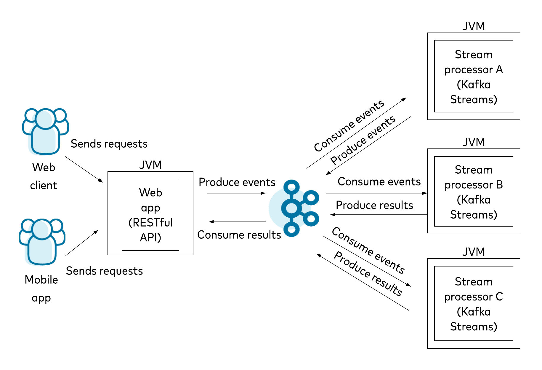 Figure 1. Example high-level architecture of an application using Kafka Streams
Event stream processing is performed on Kafka Streams application nodes; Kafka brokers do not perform any computation logic. Because of this, the same event can be processed simultaneously by multiple distinct stream processors at once. Since a stream processing platform is a distributed system, we’re going to create a separate stream processor for each type of analysis that we’ll perform. Let’s see how each of our individual stream processors fits into the general picture and what value it brings. (We’ll keep the discussion at a high level for now, but don’t worry—we’ll take a deep dive into the implementations later.)
Beginning with device recognition, our system will compare the device used in a particular login attempt against a knowledge base that stores details about each user’s previously used devices. In technical terms, we’ll use a join operator to combine an infinite login event stream with a Known Devices table representing all known user devices in a given point in time. As the system acknowledges new devices as trusted, the table will be updated as well, and its state will change accordingly. A stream is represented in the Kafka Streams API as a KStream, and a table is represented as a KTable. Both abstract the consumption of events from an underlying Kafka topic. We’ll discuss this in more detail later.
In addition to this device recognition step, our other processing stages will use stateless filtering functionality (filter and filterNot) to process only appropriate events. The location recognition stream processor will use a flow very similar to the one used for device recognition, but it will analyze different properties of login attempts. This difference will actually be the implementation of the function given as an argument to the map operator. We can then join the resulting streams from these two stream processors—New Device Attempts and New Location Attempts—in the downstream processor, which may, for example, send a message to the user, stating that their account has been accessed from a new context (device, location, or both).
For location recognition, we can track some potential malicious behaviors. As people unfortunately can’t yet teleport, we can look for rapid location changes. If we observe that a user accessed his account one hour ago in central Europe and now observe an attempt to access the same account from another continent, it seems a bit unlikely that the user really traveled such a distance in that short time. Here, we’ll apply the time windowing and aggregation functions available in the Kafka Streams API. Obviously, we cannot be 100% sure yet that a highlighted situation indicates an attack (there are also valid cases where this might be completely legitimate, such as when a user accesses their account via a VPN), but we can at least keep an eye on this account.
Botnet detection is a much broader topic. The simplest approach may be to simply check the IP address of the request. The stream processor can check whether a particular IP belongs to an IP blacklist provided, for example, by our SecOps department. We can accomplish this by joining a login event stream with a global table containing the blacklist. A global table (GlobalKTable) differs from a standard one. Bill Bejeck broadly discusses the difference in the beginning of his blog post, Predicting Flight Arrivals with the Apache Kafka Streams API.
To take this even further, we can build our own intelligence that calculates IP reputation and blacklist addresses according to our own defined rules. In order to do that, we again want to use aggregation functions, but first we would want to map and merge different types of information from other sources than the Login Attempts event stream (see the section Integration with Other Systems).
The remaining requirement of detecting brute-force attacks involves what we can observe in the context of a particular session or user. We’ll focus only on session statistics, but we could apply a similar approach when analyzing traffic from any other perspective. We can calculate session statistics for different time window configurations simultaneously. Kafka Streams offers multiple windowing options (see the documentation for details).
Last but not least, we need to join all of the knowledge gained in the previous steps and draw conclusions based on that data. The malicious login attempt stream processor will join all of the previous output streams, and then apply some business rules in order to identify malicious login attempts. As with any other stream processor, it will output results to a stream, which in this case is the Malicious Attempts stream. This stream could potentially be consumed by an authentication provider, which could act upon it by refusing to issue an access token, revoking previously granted permissions, redirecting the attacker to a honeypot, etc.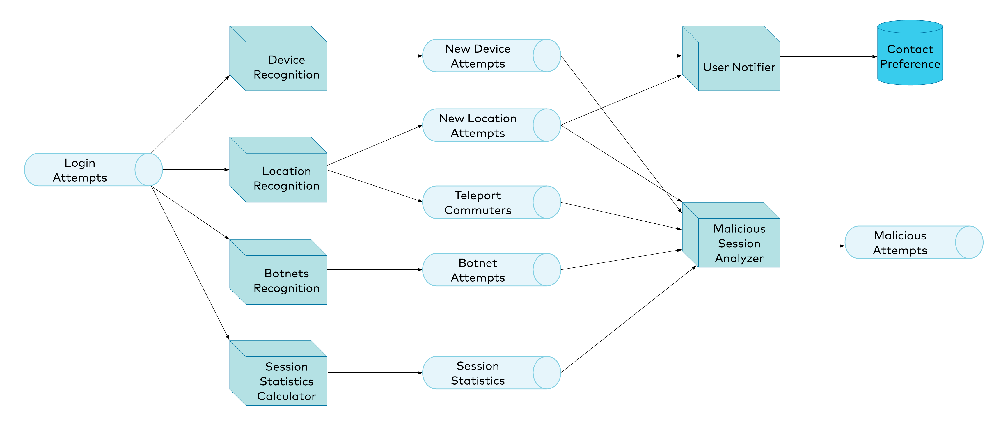 Figure 2. Risk detection platform architecture diagram
Integration with other systems
All of the analysis we have discussed so far is triggered by every single event that comes through our single source: the Login Attempts event stream. As you can imagine, in a real environment, you might want to analyze many different streams of data. Applications may publish data directly to the Kafka topics that underlie our streams. However, this isn’t always possible due to some limitations, such as lack of connectivity between Kafka and the deployment environment or just fear of touching a legacy codebase.
This is where Kafka Connect comes in handy. It is a framework that supports seamless Kafka integration with most popular datastores (both SQL and NoSQL), messaging systems, and monitoring platforms. There are multiple connectors built by Confluent or the community, which can be used to pull data from or publish data to other systems. This allows us as developers to focus on providing business value, rather than solving yet another integration problem.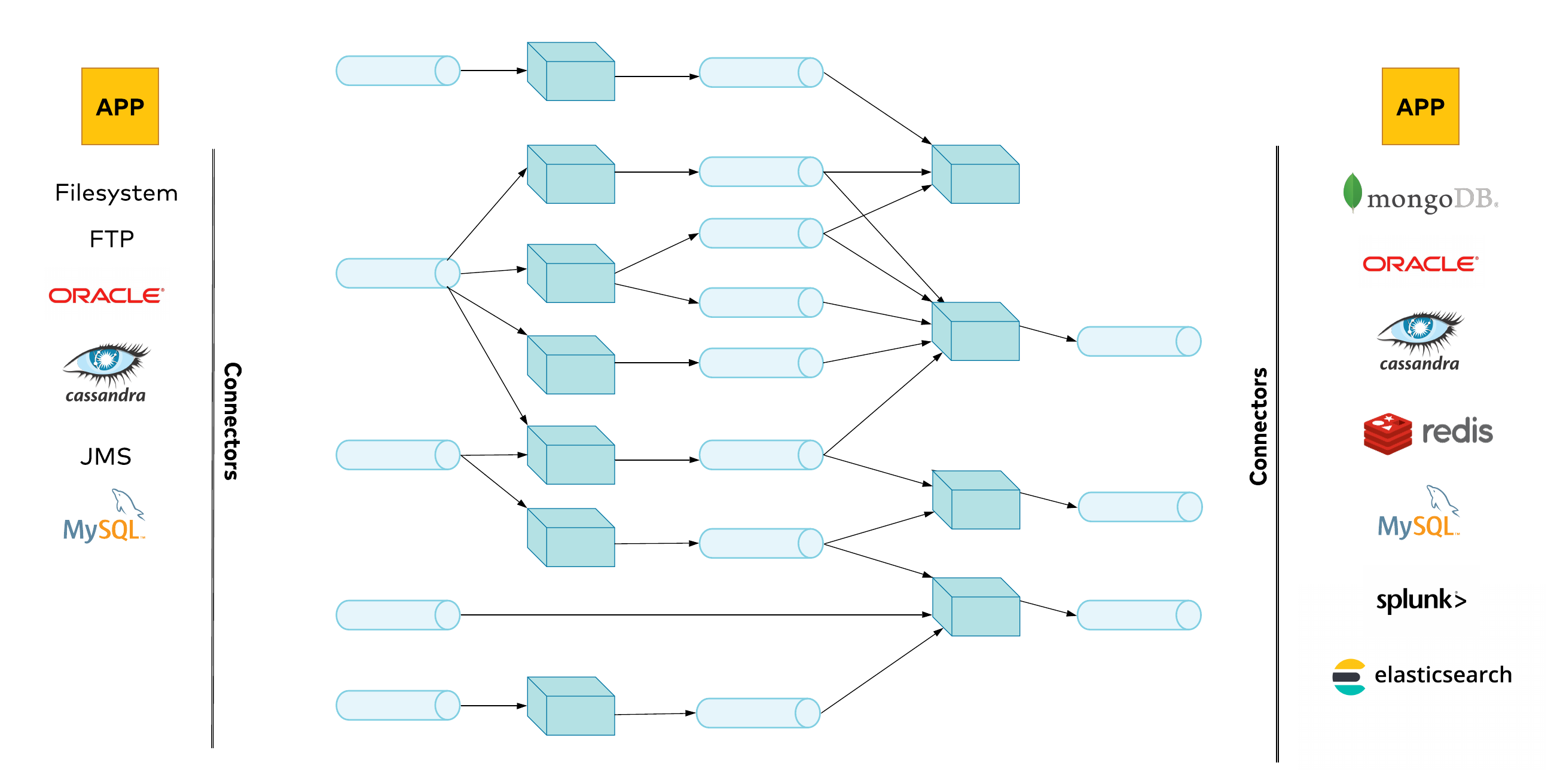 Figure 3. High-level architecture diagram, showing multiple event sources
Identity fraud detection with Kafka Streams
Let’s take a close look at how we’ll build the device recognition feature.
We’ll take our implementation through several iterations. Our first design is based on the assumption that because we have two separate outcomes from our processor, we can divide our work into two separate units of work, which can run in parallel: New Device Attempts and Known Devices. The computational logic behind each of these units of work is what we call a topology. Both topologies are triggered by every event in the Login Attempts stream.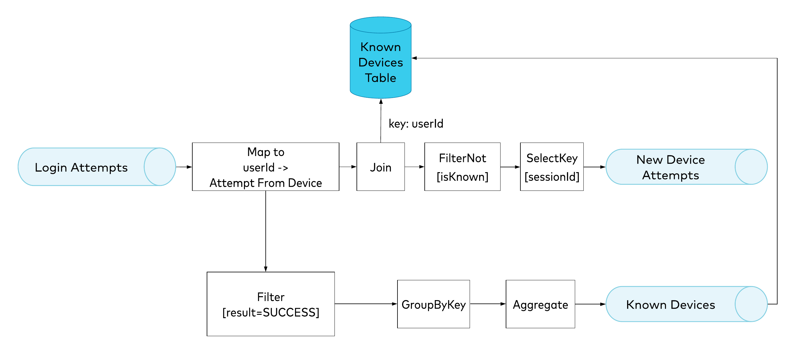 Figure 4. Initial design, with two independent topologies
As we can see in the topology diagram (Figure 4), the first event streaming operator we apply is map, which just converts one event to another. In our case, it will switch the key of an event from sessionId to userId, strip out all unused properties, and calculate the hash based on the properties that we consider most important for the device. It is the result of the map operator that triggers the two topologies.
| Login attempts | Intermediate events after mapping | |
| Key | sessionId (xyz) | userId (abc123) |
| Payload |
{
  event: {
  result:SUCCESS/FAILURE,
  userId: "abc123",
  timestamp: 987654
 },
 metadata: {
   device: {
     os: "Mac OS",
     browser: "Chrome/76.0.1",
     platform: "MacIntel",
     timezone: "UTC+2",
     language: "PL"
   },
   geolocation: {
     …
   },
   network: {
     …
   }
  }
}
|
{
  result: SUCCESS/FAILURE,
  timestamp: 987654,
  device: {
    hash: "cvxsk4",
    originSessionId: "xyz",
    os: "Mac OS",
    browser: "Chrome/76.0.1",
    platform: "MacIntel",
    timezone: "UTC+2",
    language: "PL"
  }
}
|
Table 1. Events before and after use of the map operator
We consider a device as a known device if it has been used at least once in a successful login attempt. Thus, when building our knowledge base of a user’s known devices, we need to only consider successful login attempts. This is why we need to apply the filter operator, which removes from the stream all events that do not match a defined predicate. The filtered stream is then grouped by a key (userId) in order to be aggregated. Unlike other operators in the pipeline, aggregate is stateful: it accepts the trigger event together with the previous version of the aggregate and combines them. In our case, it just adds the device from the attempt that we’re analyzing to the collection of the user’s known devices.
All that’s left now is to detect whether the device used in the currently analyzed attempt is already known. To perform this check, we need to use the information from the Known Devices pipeline. We will use the join operator for this purpose. The left side of the join is an intermediate remapped stream of login attempts; the right side is the Known Devices table. When you consume a stream, you are interested in each event independently as it occurs, whereas a table reads the stream and treats every event with the same key as an update, and thus represents the current state of the world. In our use case, we would like to know the latest version of the Known Devices aggregate, so our New Devices pipeline will consume the aggregate as a table. There is a duality between the two: you can always convert from a stream to a table, and vice versa. This particular topic is extensively described by Michael Noll in his post, Streams and Tables in Apache Kafka: A Primer.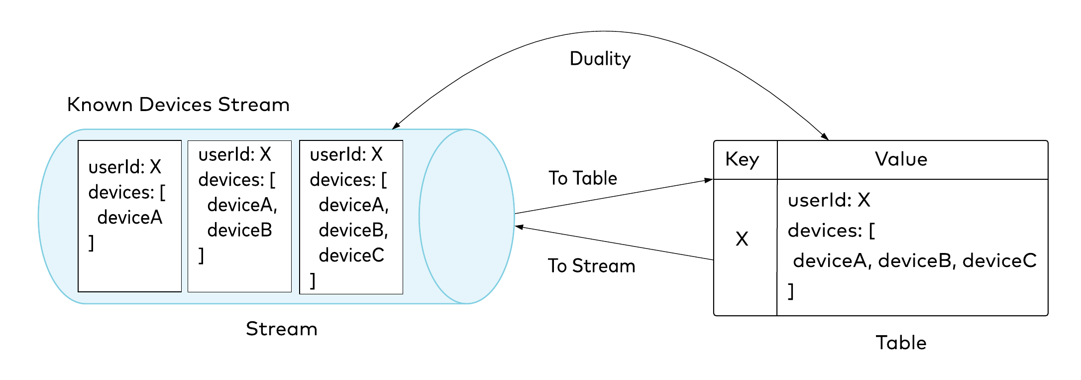 Figure 5. Stream-table duality
Getting back to the topology—just after performing the join, we can finally determine whether or not the device is already known. With this knowledge, we will enrich the intermediate event with some marker field, such as isKnown, which will hold a Boolean value. We will check this field in the predicate of the next operator in our pipeline: filterNot. This step will exclude attempts from already-known devices. Our last operator, selectKey, just switches the key back to sessionId for further analysis. Finally, we send the events to the New Device Attempts topic.
Our topology is complete, but a few more words about the join operator are in order. In the world of relational databases, joins can be quite expensive, especially when handling high volumes of traffic. Yet we’re using joins in this topology. Why?
Co-partioning
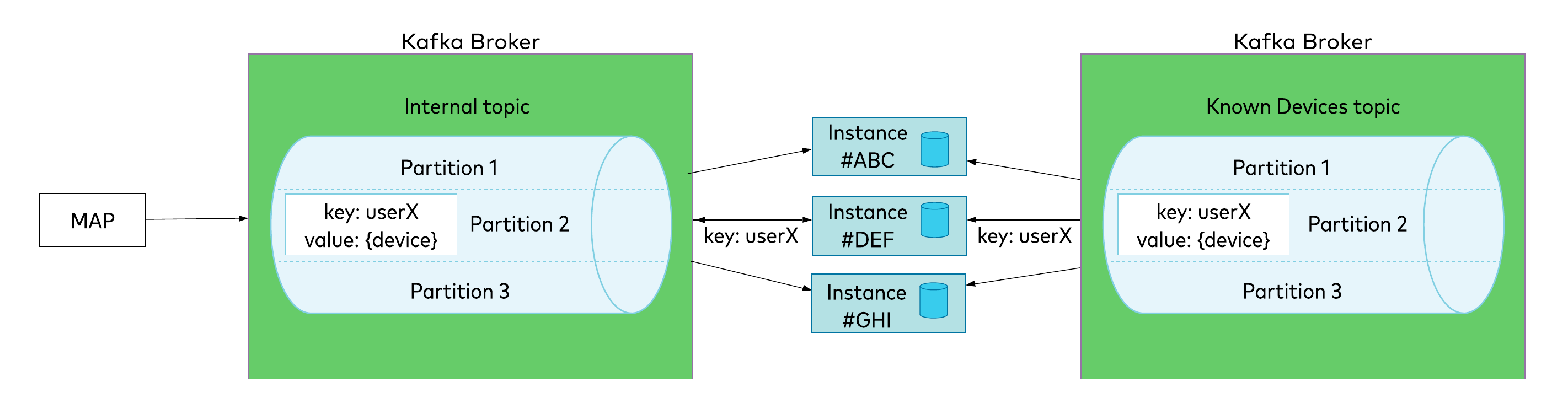 Figure 6. Joining two co-partitioned topics
Well…because joins work a bit differently in Kafka.
To understand how a join works, let’s first look at how an event is published to a topic in Kafka. Each Kafka topic has multiple partitions, and the partition number is a unit of parallelism: only one consumer in a given consumer group can consume a partition. When an event is published, the producer gets the key of the event, applies the hashing algorithm to it, and writes an event to a calculated partition number. Every subsequent event with the same key is guaranteed to be put in the same partition. This partition is then assigned to one of the processing nodes when it starts up.
Now, if different topics within a single processing pipeline have the same partition count, we can be sure that partitions with corresponding numbers will be assigned to the same processing instance. As shown in Figure 6, events for userX from both topics will be consumed by instance #DEF. When consuming a subsequent login attempt from the stream on the left, the processing instance will already have the aggregate stored locally. Depending on the configuration, the join—which always relies on the key—is in fact just a matter of in-memory or local persistent storage lookup. (By default, Kafka Streams uses RocksDB, which keeps data in persistent storage, but as of Kafka 2.4, you can implement your own strategy for keeping the state store. In other words, you might keep it in a database, a cache, or even a hash map.)
These characteristics help us ensure data locality. There is no need for any remote calls, as we have everything we need in the processing node’s memory. Data locality is very important when building systems that have a high volume of traffic and must have low processing latency. The key here is to keep relevant data close to the computation.
Race condition!
Our first design is quite simple: two independent topologies, with one supplying data to the other. Unfortunately, this design has an important flaw. Up to this point, we haven’t enforced the execution order of our topologies. Because the system is distributed and asynchronous, we cannot make any assumptions about it. It’s possible that for a successful login attempt, the Known Devices topology finishes even before the New Device Attempts topology kicks in. The latter may experience some processing lag because of downtime, for example, and it will need time to catch up. If this occurs, the Known Devices state store may have been updated even before it started analyzing a particular login attempt, so the result of the join will be incorrect and indicate that the device is already known. How can we solve this issue?
A refined design
When we think about our requirement that a new device should be recognized as known only if it has been used in a successful login attempt, it seems reasonable to first recognize an attempt as coming from a new device, and only append it to the Known Devices aggregate if the current attempt succeeds. In other words, we’re introducing a dependency between our topologies. An event in the New Device Attempts stream will trigger the Known Devices pipeline. Because of this dependency, we can be sure that we won’t update the Known Devices table before analyzing a particular login attempt. Problem solved!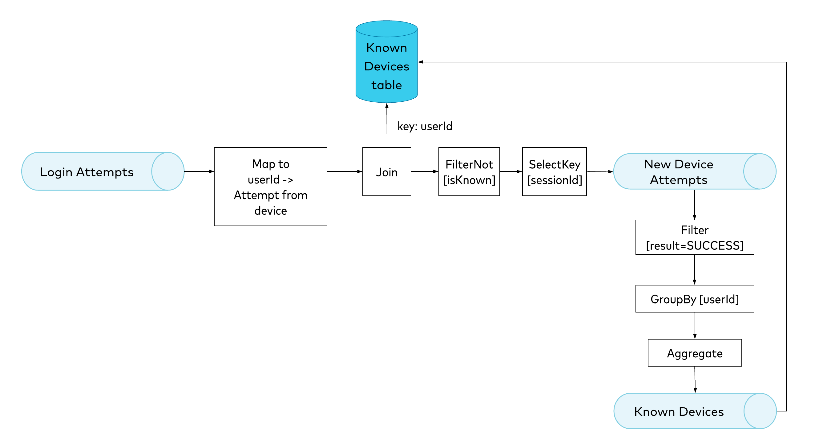 Figure 7. Refined design, reorganizing the topologies
This approach should work fine for our current use case. But if we imagine a hypothetical situation in which some small number of our users are accessing the system using thousands of different devices (location recognition is probably a more realistic example here), the Known Devices aggregate becomes quite large. This might lead to a data skew effect, with a few aggregates becoming significantly larger than the rest. We definitely don’t want this effect, and it would be quite difficult to trace and fix it in a live environment. Let’s see how we can eliminate this issue in our final design.
The final design
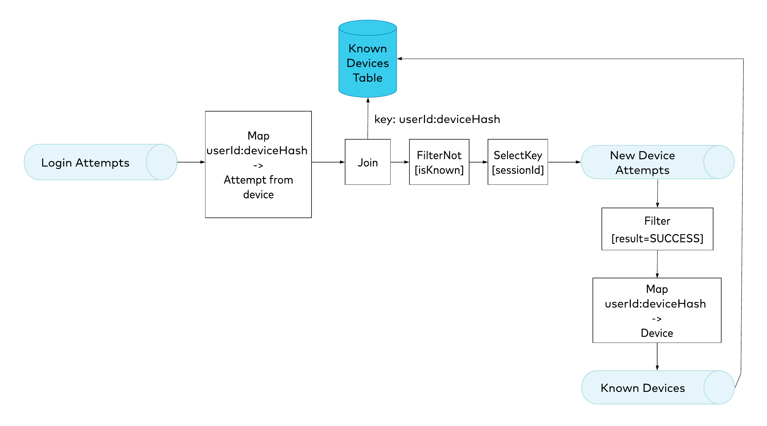 Figure 8. Final design, using composite keys
No one has ever claimed that a key in Kafka should be only a single-value string. Actually, a key can be any type of object, since Kafka just stores it as bytes and doesn’t care what’s inside. This means that here, we can use a composite key. In production, you would most likely want to use an Apache Avro™ key, which, together with the Confluent Schema Registry, can protect the compatibility of the schema. In this example, just for simplicity, we’re going to use a string composite key that concatenates two properties. Until now, we’ve been using userId as a key for the Known Devices aggregate. In our final approach, we will concatenate the userId with the device hash.
Let’s look first at the changes we’re making to the Known Devices topology. The filter operator stays the same, but now there’s no grouping and aggregating. Instead, we now map the New Device Attempt to an event that has a composite key (the userId and the device hash), with the device object as a value. We’re changing our strategy: instead of giving the Known Devices table one row that contains an aggregate with the collection of the user’s known devices, we now will store multiple rows, each representing a different user’s device.
| Value | Key |
| userX:234abc |
{
  os: "Mac OS",
  browser: "Chrome",
  platform: "MacIntel",
  timezone: "UTC+2",
  language: "PL"
}
|
| userY:qwe544 |
{
  os: "Android",
  browser: "Chrome",
  platform: "Mobile",
  timezone: "UTC+1",
  language: "EN"
}
|
| userX:bnm876 |
{
  os: "Windows",
  browser: "Firefox",
  platform: "Intel",
  timezone: "UTC+2",
  language: "EN"
}
|
Table 2. Contents of the Known Devices table
With this strategy, we will need to use the same key for the join in the New Device Attempts topology. The first map operator must set the exact same composite key. After performing the join, we no longer need to check whether the collection stored in the aggregate contains a new device. If the join result is not null, we know immediately that we haven’t seen this user and device combination before. Otherwise, the device is known and trusted.
By organizing our topologies in this way, we have optimized the whole processing pipeline, removing the stateful aggregate operator. This helps us to reduce memory usage on processing instances and also saves us some bandwidth, since we’re sending smaller events over the network.
One very important note as we close: a distributed system such as this requires detailed analysis. As we’ve seen, it’s fairly easy to run into different types of problems unless we start with a proper design.
Summary
This article has illustrated how you can apply the stream processing paradigm to build software that provides results in real time and at scale. Together with ksqlDB (another great way to build stream processors), features in the Kafka Streams framework help engineers to focus on delivering real business value.
If you’d like to learn more, you can watch my Kafka Summit session or listen to this episode of the Streaming Audio podcast hosted by Tim Berglund.


