Streams and Tables in Apache Kafka: Elasticity, Fault Tolerance, and Other Advanced Concepts
Now that we’ve learned about the processing layer of Apache Kafka® by looking at streams and tables, as well as the architecture of distributed processing with the Kafka Streams API and ksqlDB in part 3, we will revisit the processing layer again and dive into how elastic scaling and fault tolerance are architected and implemented—including a return to the stream-table duality, which turns out to underpin many of these capabilities.
Let’s start with how fault-tolerant processing of streams and tables is achieved, after which we will explore elasticity. We’ll see that these subjects are actually two sides of the same coin.
- Streams and Tables in Apache Kafka: A Primer
- Streams and Tables in Apache Kafka: Topics, Partitions, and Storage Fundamentals
- Streams and Tables in Apache Kafka: Processing Fundamentals with Kafka Streams and ksqlDB
- Streams and Tables in Apache Kafka: Elasticity, Fault Tolerance, and Other Advanced Concepts (this article)
Fault-tolerant processing
Streams and tables are always fault tolerant because their data is stored reliably and durably in Kafka. This should be relatively easy to understand for streams by now as they map to Kafka topics in a straightforward manner. If something breaks while processing a stream, then we just need to re-read the underlying topic again.
For tables, it is more complex because they must maintain additional information—their state—to allow for stateful processing such as joins and aggregations like COUNT() or SUM(). To achieve this while also ensuring high processing performance, tables (through their state stores) are materialized on local disk within a Kafka Streams application instance or a ksqlDB server. But machines and containers can be lost, along with any locally stored data. How can we make tables fault tolerant, too?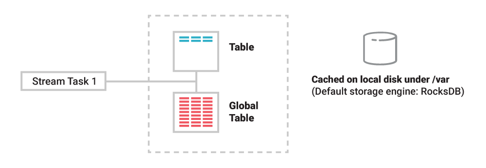
Figure 1. Tables and other state are materialized (cached) by stream tasks to local disk inside your Kafka Streams applications or ksqlDB servers.
The answer is that any data stored in a table is also stored remotely in Kafka. Every table has its own change stream for this purpose—a built-in change data capture (CDC) setup, we could say. So if we have a table of account balances by customer, every time an account balance is updated, a corresponding change event will be recorded into the change stream of that table.
Similar to a redo log in a relational database, this change stream is the source of truth for the respective table, and it is continuously and durably stored in a Kafka topic—its so-called changelog topic. This means that fault tolerance is achieved by exploiting the stream-table duality we discussed in the first article of this series. Whatever happens to the stream task or the container/VM/machine it is running on, a table’s data can always be correctly restored from its change stream, via the changelog topic, so that processing can resume without data loss or incorrect processing results.
If a container failure means that our account balances table needs to be rebuilt on another container, then we don’t need to rerun the whole process (i.e., replay all payments and recalculate all balances). We can simply restore the state of the table as it was when the failure happened directly from the changelog topic. Changelog topics are also compacted, so this is a very efficient process as we will see later.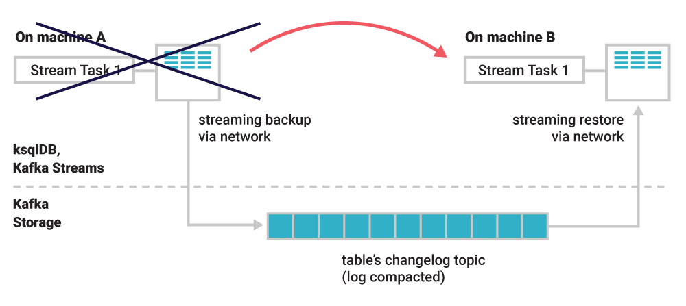
Figure 2. A task runs on machine A. The (partition of the) table it uses is continuously backed up into a Kafka topic. If machine A dies, the task will be migrated to another machine. There, the table will be restored to exactly the state it was when the task stopped on the original machine. Once the restoration is complete, the task will resume processing on machine B.
Elastic processing and scalability
The previous section on fault tolerance is a great segue into elasticity. What a distributed system needs to do to handle unexpected failures (such as a lost container) is remarkably similar to what it must do to achieve elasticity (like scaling your application out by adding containers, or scaling in by removing containers). It doesn’t really matter whether a container was removed intentionally or by failure. In other words, elasticity and fault tolerance are two sides of the same coin!
Imagine running two instances of a Kafka Streams application. Their input is a topic with four partitions, hence there will be four stream tasks. These four tasks are evenly distributed across the two app instances. If we now add a third and fourth app instance to scale out the application, some of the tasks including their table partitions will migrate to the new instances to share the processing load.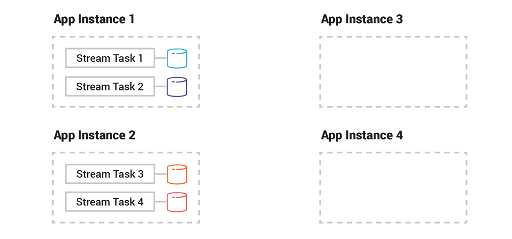
Figure 3. Task distribution of a Kafka Streams application prior to adding a third and fourth application instance to scale out
The processing logic (which filters, transforms, joins, aggregates, etc.) doesn’t require migration because it is already available to every app instance as it’s included in the packaged application binary. The only thing to do is to quickly and reliably migrate all the table data (i.e., the application state), whether it’s a few kilobytes or many gigabytes of data, using the previously described process that restores a table from its Kafka changelog topic at a target destination. The converse happens if we remove an application instance when scaling in: its tasks and tables migrate to the remaining live instances, using the Kafka storage layer as the conduit.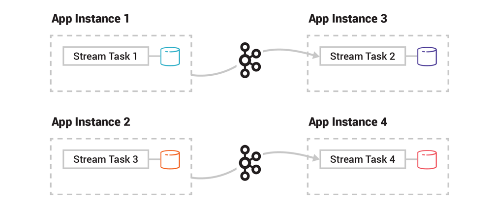
Figure 4. Task distribution of the Kafka Streams application after the scale out is completed
Every migration step described above happens automatically, which greatly reduces the burden on application developers and operators. What’s more, this elastic scaling of your applications can be done during live operations at runtime, unlike many other stream processing frameworks, where such capacity changes require fully stopping, reconfiguring, and resubmitting processing jobs.
Tables and topic compaction
Generally speaking, a table’s underlying topic is compacted. An exception to this rule is when you, for example, use ksqlDB to create a table from an existing Kafka topic, in which case any topic settings including compaction will not be modified. Compaction is a storage feature of Kafka that ensures Kafka will always retain (at least) the last event for each event key within a topic partition, as shown in Figure 5. It reduces the storage footprint of a table’s change stream in the Kafka brokers by periodically purging old events for the same event key from storage (e.g., cities that Alice visited previously in the example below).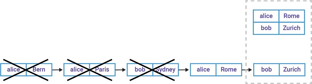
Figure 5. Compaction periodically removes older events for the same event key. The bottom half shows the table’s changelog topic (change stream) including events already removed by compaction. The top half shows the current state of the table, with the latest data for Alice and Bob.
So what’s the benefit of compaction? It allows us to store table data forever in Kafka as the permanent system of record without the data growing out of bounds. This is a great fit for reference data, such as customer profiles, a product catalogue, account balances, dimension tables, and so on. Take Kafka Connect, which uses compacted topics to durably store its configuration settings.
The second benefit is that compaction reduces the application recovery time during rebalancing because less data must be transferred over the network from brokers to ksqlDB servers or Kafka Streams applications, which improves elasticity and failure handling. Imagine having a table of 1 million customers. This table sees many changes throughout the day, totaling 400 million total change events thus far. With compaction enabled, restoring the table of customers is much faster because it only needs to read the latest 1 million events from the table’s change stream instead of the full 400 million.
Compaction is thus very useful. That said, please note that compaction intentionally removes part of a table’s history—the crossed-out events in Figure 5. If you do need its full history but don’t have the historic data elsewhere, such as in another stream from which the table was generated, then consider disabling compaction. And for what it’s worth, you should never enable compaction for streams because here, new events for the same key should not be interpreted as “superseding” prior events!
Operational aspects of elasticity and fault tolerance
What underlies failure handling and elasticity is Kafka’s rebalancing process, which we have already covered in detail above. What we need to understand for running our Kafka Streams applications and ksqlDB setups in production is that there will be a period of time—typically small—during which a part of an application will be unavailable until the rebalancing is complete. For ksqlDB and Kafka Streams, this is the time it takes to fully migrate any impacted tasks along with their tables and any other state.
The more table data that needs to be restored for a migrated task, the longer the recovery time. For example, the network bandwidth between a client-side application instance (where a table partition needs to be restored to) and a server-side Kafka broker (which hosts the topic partition from which to restore the table partition) may become a limiting factor if lots of data must be transferred.
The aforementioned compaction feature (enabled by default) is pretty effective at reducing the amount of data that needs to be transferred during task migration. Another very useful feature that you can use with both ksqlDB and Kafka Streams to minimize the recovery time for (a) failure and (b) scale-in scenarios (but not scale out) is enabling standby replicas. This setting is optional but recommended for production.
Using Kafka Streams as the example, application instances can be configured to maintain passive replicas of another instance’s table data. Think: the table partitions of one app instance will be continuously restored to a configurable number of other instances just in case. Whenever an application instance dies or is terminated, its tasks will migrate to one of the instances that already have a replica of the data, which significantly speeds up the end-to-end recovery time. The drawback of standby replicas, however, is increased network communication between app instances and the Kafka brokers and, for the app instances, increased local storage consumption because of the additional replicated table data.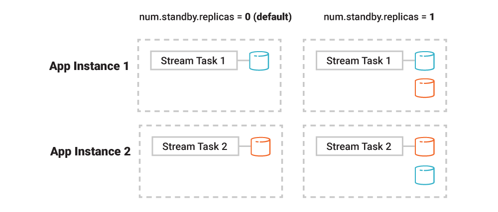
Figure 6. Standby replicas are disabled by default. If enabled, tasks will maintain additional replicas for table data (on the right: one such replica per task is shown).
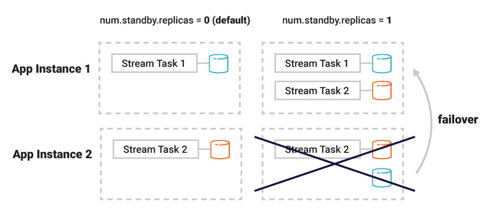
Figure 7. With standby replicas (right side), when app instance 2 is terminated along with the stream task it is running, the remaining instance 1 can quickly take over the former’s processing responsibilities because it already has the relevant table data available locally. This minimizes failover times.
Beyond what I described above, the Kafka community has been working on several improvements to make the inner workings of elasticity and fault tolerance even faster and more efficient. These are part of Apache Kafka 2.4 and the upcoming release of Confluent Platform 5.4, including the introduction of static consumer group memberships for reducing the application downtime caused by excessive and unnecessary rebalances, and incremental cooperative rebalancing for providing a much smoother scale in/out experience, notably for deployments in the cloud or on Kubernetes.
Lastly, let me share a practical tip for capacity planning: when estimating the local storage footprint of table data, don’t forget to take into account that, because of the aforementioned setup for elasticity and fault tolerance, stream tasks including their respective table partitions may be moving around at runtime across any Kafka Streams application instances or ksqlDB servers. For example, if the expected total table data is 50 GB and you run five application instances, then giving each just 10 GB of local storage is likely not sufficient—an instance would not be able to take over the work from the other four instances in the case of failure.
Partitions and processing parallelism
The maximum level of processing parallelism in Kafka is bounded by the number of partitions of the input data, be it a stream, table, or topic. If there are 20 input partitions, for example, there will be exactly 20 stream tasks. This means you can run from one up to 20 Kafka Streams application instances (or 1–20 ksqlDB server nodes in a ksqlDB cluster), across which the stream tasks will be distributed evenly. Any surplus application instances, however, will stay idle.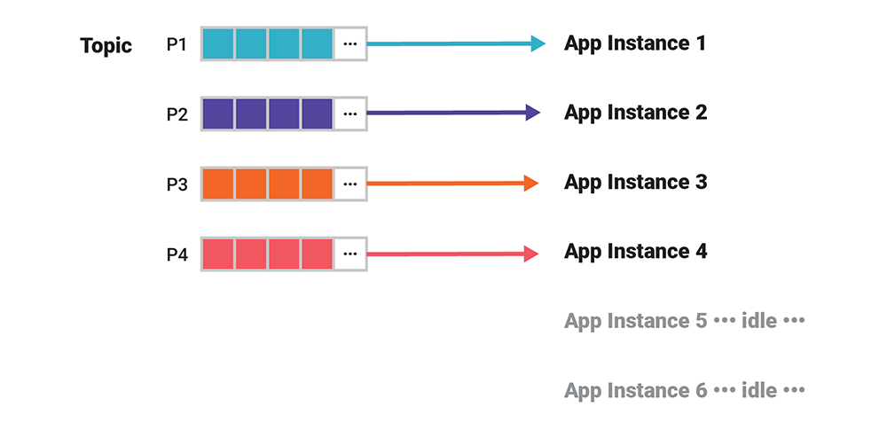
Figure 8. The level of parallelism cannot exceed the number of input partitions. You can launch additional application instances, but they will stay idle. If you have fewer instances than partitions, then multiple partitions will be allocated to individual app instances.
But what should you do if you need to increase the level of processing parallelism? If you need higher parallelism in general, then you must increase the stream’s or table’s partition count. Existing applications will need special care because, most likely, events are now being sent to different partitions than before (see same event key to same partition from part 2 of this series). If you need higher parallelism for just one use case, you can often leave the original stream/table as is and instead derive a new stream/table from it that has a higher partition count. You can also consider lowering its retention to save storage.
Here is the code example in ksqlDB:
Dealing with data skew
Speaking of parallelism and processing speed, you may run into a situation where some stream tasks are getting overwhelmed with work, whereas others have little to do. The best way to spot this is through proper operational monitoring of relevant metrics, such as consumer lag.
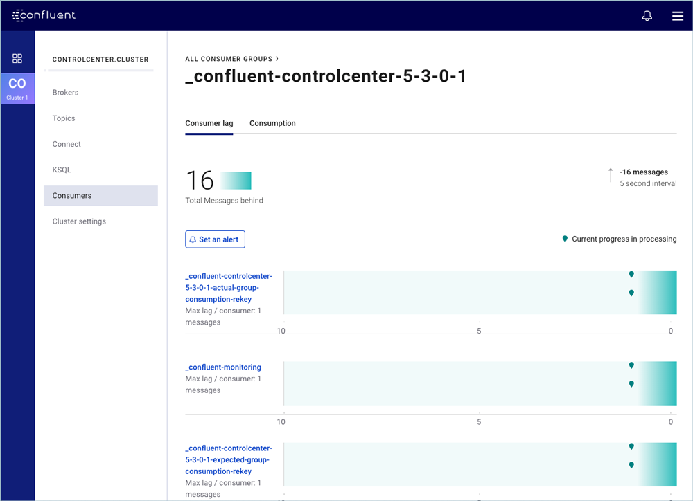
Figure 9. Consumer lag monitoring with Confluent Control Center
The following table shows the two most common causes of data skew together with their respective remedies.
| Cause | Solutions |
| Storage skew: Events are unevenly distributed across partitions. The few partitions that take the majority of the events are called hot partitions. See Figure 10. |
Data ingress: Find a better partitioning function such as ƒ(event.key, event.value) for producers so that new events are more evenly distributed as they come in.
Storage: Re-partition the existing events into a new topic with a larger number of partitions. See the ksqlDB code example at the end of the previous section. |
| Processing skew: Events are evenly distributed but certain events take significantly longer to process. | Scale processing vertically, including using more powerful CPU instances. |
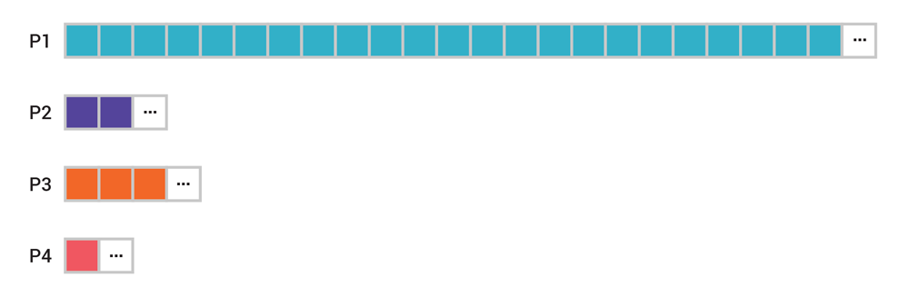
Figure 10. Skew in your data may lead to hot partitions (in this case, P1). Data generated in scale-free networks like social networks, whose degree distribution follows a power law, are but one example where this may happen in practice.
Capacity planning and sizing
For more details on capacity planning and sizing, please refer to ksqlDB Capacity Planning and Kafka Streams Capacity Planning. If you prefer this information in video format, I recommend the talk ksqlDB Performance Tuning for Fun and Profit (abstract) from Kafka Summit San Francisco 2019.
Summary
This completes the fourth and final part of this series. If you made it this far, well done—I think we covered quite a bit of ground together! We started with a primer in events, streams, and tables, and then walked through the bits and pieces of Kafka’s storage layer all the way up to Kafka’s processing layer with tools like ksqlDB and Kafka Streams that allow you to build applications and process events as streams and tables. Finally, we covered how these applications are made to be elastic and fault tolerant.
I hope this four-part series leaves you with an understanding of event streaming with Apache Kafka, and what you need to watch out for when putting events, streams, and tables to practice in your own applications and use cases.
Interested in more?
If you’d like to know more, you can download the Confluent Platform to get started with a complete event streaming platform built by the original creators of Apache Kafka.
Previous articles in this series
このブログ記事は気に入りましたか?今すぐ共有
Confluent ブログの登録


Why ELT Can't Keep Up in the Era of High-Scale Data Engineering
Batch ELT pipelines create duplication, cost spikes, and governance gaps as data scales. Here’s why enterprises are rethinking legacy integration models.


How to Protect PII in Apache Kafka® With Schema Registry and Data Contracts
Protect sensitive data with Data Contracts using Confluent Schema Registry.