Neu in Confluent Cloud: Daten & Pipelines für KI-fähiges Streaming zugänglich machen | Mehr erfahren
Apache Kafka and R: Real-Time Prediction and Model (Re)training
Machine learning on real-time data is a powerful combination because you gain direct insights into your data, can make powerful decisions, and consequently improve your business processes and outcomes. It is important to know how to implement the statistical model into your running system as well as how to deal with data value changes and decreased prediction results.
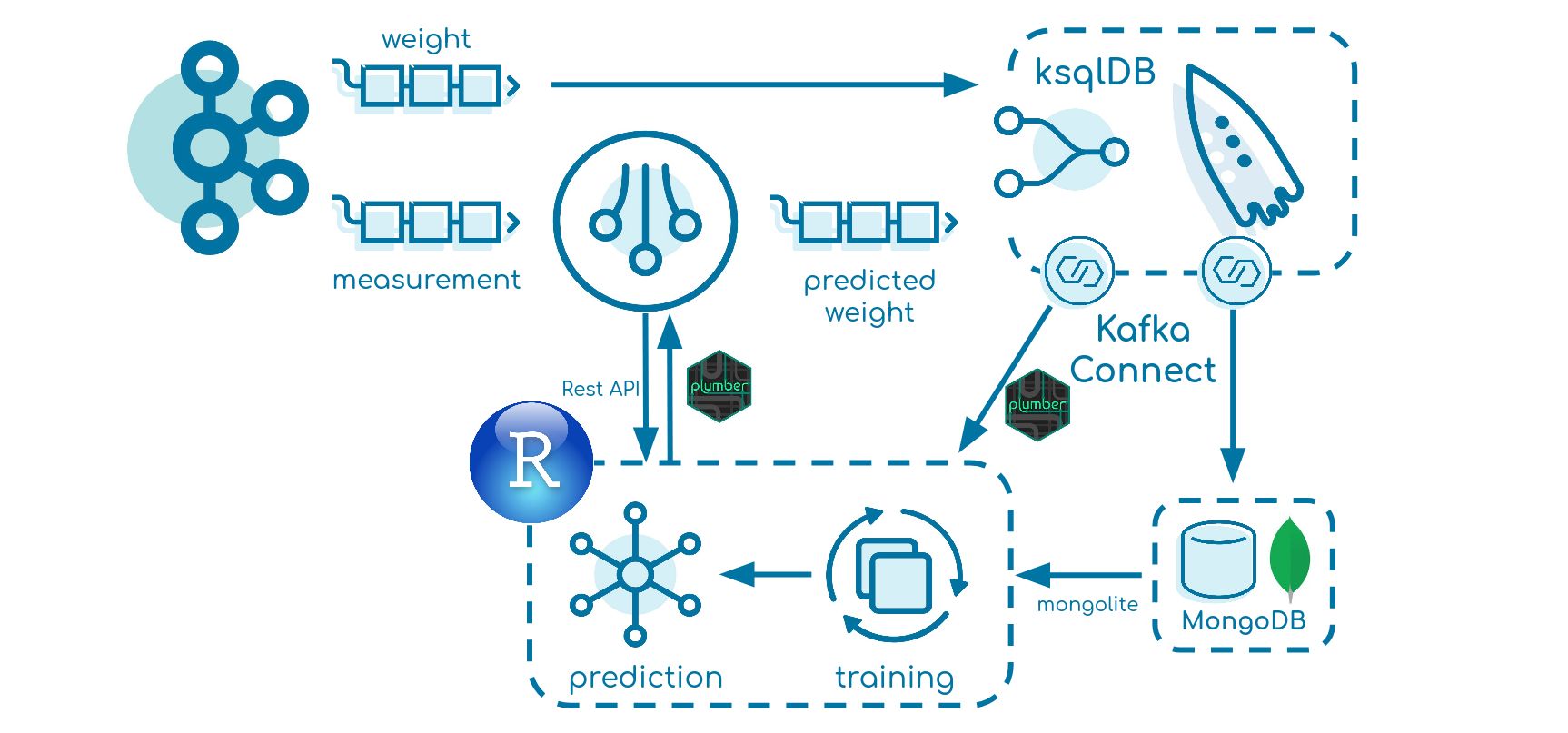
This blog post creates a data pipeline in which a machine learning model is applied and also automatically retrained once the prediction results exceed a certain threshold. Simulated data is used to highlight certain key characteristics of the data flow. More specifically, a Kafka Streams application (implemented with Kotlin) will send an HTTP request to the model (implemented in R using the plumber package) and produce the prediction back into a sink topic. Finally, ksqlDB, as well as a MongoDB Connector and HTTP Sink Connector, is used to store data and to trigger the retraining process.
This tutorial goes through the build and also talks about testing key implementations. Furthermore, an overall pipeline performance scan, as well as insight into the drawbacks and limitations, complement this article.
Note, this article does not focus on data science itself, such as choosing and optimizing the statistical model. The overall goal is to transfer the model into the running system, focusing on simplicity so that the guideline can be used as a basis. A subsequent article about optimization is planned for the future.
All code used in this article can be found on GitHub.
The simulated business case
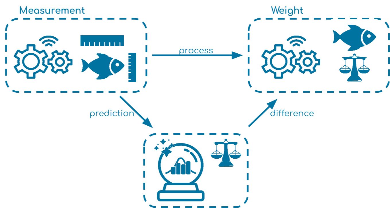
The generated example used a factory for fish processing. In the first step, the fish size (length and height) is measured. Later in the process, the fish is also weighed to calculate the amount of meat and finally to define the price.
It is assumed that the size of the fish may have an impact on the weight—the bigger, the heavier—so it would be great to approximate the weight directly so that we can tell the customer what the next charge might cost in advance.
Dimensions.com provides fish information about many species, so we can simulate a data set of 100 salmon fish with height, length, and weight. The data is used to train a simple linear regression model with the command lm(weight ~ length + height, data = data). The model itself is significant and explains 83% of the data’s variance. The data is saved to use later in our pipeline with the command save(data = lm, file = "model.RData"). The analysis can be found in the file Model.R.
Simulated IoT devices
Two Kafka producers representing both machines send data into the topics machine-measurement and machine-weight in JSON format every two seconds continuously. The events for the measurement and the weight look like this:
{
"Species": "salmon",
"Fish_Id": "1",
"Length": 86.370,
"Height": 18.740
}

{
"Species": "salmon",
"Fish_Id": "1",
"Weight": 4.43990
}
The weight producer sends its data with ten seconds delay to simulate the consecutive process.
Model API
RStudio is used to apply and retrain the model. Both functions can be found in the file Predictor.R. To create an API we use the plumber package and define its port and host in main.R.
library(plumber)
api <- plumb("/home/Predictor.R") api$run(port=8000, host="0.0.0.0")
There are several articles about creating an API with the plumber package and running it with Docker, including R can API and So Can You! and Using docker to deploy an R plumber API, written by Heather Nolis and Jacqueline Nolis.
Prediction function
For prediction, we define a GET request having the length, weight, and species as parameters.
#' @param length
#' @param height
#' @param species
#' @serializer unboxedJSON
#' @get /prediction
predictWeight <- function(length, height, species){

  tryCatch(
	{
  	length <- as.numeric(length)
  	height <- as.numeric(height)
  	species <- as.factor(species)

  	load("/home/model.RData")

  	prediction <- predict(lm, data.frame(length = length, height = height, species = species))
  	return(list(Weight = prediction, ModelTime = lm$time))
	},
	error = function(cond){
  	message("Prediction did not work")
  	return(NA)
	}
  )
}
We transfer the input parameters, apply the trained linear regression model, and return the prediction as a JSON object:
{
"Weight": 3.6789,
"ModelTime": "2021-06-02 07:48:52"
}
Retraining function
We define a POST request to retrain the model.
#' @post /train
train <- function(){
  library(mongolite)
  library(dplyr)

  tryCatch({
	connection <- mongo(collection = "TrainingData",
                    	db = "Weight",
                    	url = "mongodb://user:password@mongo:27017")
   	dataAggr <- connection$aggregate('[
            	{"$sort": {"Timestamp": -1}},
            	{"$limit": 50}]')
 	data <- dataAggr %>% select(length = Length, height = Height, weight = ActualWeight, species = Species)

	if(length(unique(data$species)) > 1){
  		data$species <- as.factor(data$species)
  		lm <- lm(weight ~ length + height + species, data = data)
	} else {
 	  	lm <- lm(weight ~ length + height , data = data)
	}
	lm$time <- Sys.time()
	save(data = lm, file = "/home/model.RData")
	message("New model saved")
  },
  error = function(cond){
	message ("Retraining did not work")
	}
  )
}
Using the mongolite package as well as the dplyr package, we first request the last 50 data points out of MongoDB and then transfer them into our desired form. In this previous article, Create a Data Analysis Pipeline with Apache Kafka and RStudio, a data pipeline is created from Apache Kafka® into R using Kafka Connect and MongoDB. Subsequently, we apply our model conditioned on the number of species and save it.
Testing
To test whether the API is working as expected we run a docker-compose file in the directory /R/test. This one starts the plumber API, a MongoDB container, and inserts data into the database. On http://127.0.0.1:8000/__docs__/ you can find an interactive Swagger page on which you can directly test your API. In this running example the following behavior is tested:
- GET request to test if the prediction works in general ✔
- POST request to retrain the model ✔
- GET request to test if the model time has changed due to retraining ✔
Even though we test our API in an integration test, we also need to think about unit tests. This step is omitted in this tutorial, but you can refer to the testthat package as well as to the article Unit Testing in R by André Müller which explains unit testing in R very well.
Real-time prediction
For the prediction, we implement a Kafka Streams application in Kotlin using Kafka Streams version 2.8.0. The application has the following properties:
BOOTSTRAP_SERVERS_CONFIG: “broker:29092”,
APPLICATION_ID_CONFIG: “streamsId”,
MODEL_URL: “http://rstudio:8000/prediction”
We just set the mandatory configuration parameters and we specify the model URL. At this point, we only focus here on the topology as well as the interaction with the model in RStudio because that’s of main interest. For serialization and deserialization of Kafka events, we implement a customized FishSerde using the Klaxon library.
Topology
class StreamProcessor(properties: StreamProperties, private val predictor: Predictor) {

   val streams = KafkaStreams(createTopology(), properties.configureProperties())

   fun createTopology(): Topology {
       val processor = StreamsBuilder()
       processor
           .stream(
               "machine-measurement",
               Consumed.with(Serdes.String(), FishSerde())
           )
           .filter { _, value -> value != null }
           .mapValues { value -> predictor.requestWeight(value) }
           .to(
               "weight-prediction",
               Produced.with(Serdes.String(), FishSerde())
           )
       return processor.build()
   }
}
The topology is straightforward: consume the topic machine-measurement, filter out null values, apply the prediction within the mapValues transformation, and finally produce the result back into the sink topic weight-prediction. For more information about stateless and stateful transformations, see the Kafka Streams documentation.
API communication
To send the GET request, we use the Ktor library.
fun request(fish: Fish, url: Url): Any? =

   runBlocking {
       val client = HttpClient(CIO)

       try {
           val response: HttpResponse = client.request(url) {
               method = HttpMethod.Get
               parameter("length", fish.Length)
               parameter("height", fish.Height)
               parameter("species", fish.Species)
           }
           client.close()
           return@runBlocking response.readText()

       } catch (e: Exception) {
           logger.error("Could not receive a weight for payload: $fish to url: $url")
           return@runBlocking null
       }
   }
}
We set up a HttpClient and send the GET request to the desired URL with additional parameters. For a successful request, we return a JSON string that needs to be parsed to an object; for a failed request we return null.
Testing
When testing in Kotlin, we usually use Kotest as well as Mockk for mocking objects. At this point, we only focus on testing the topology even though there is an integration test for the API communication provided in the file PredictorIntTest.kt.
We use the ToplogyTestDriver for testing the Kafka Streams topology.
class StreamProcessorTest : StringSpec() {
   private val input = Fish("id", "salmon", 1.0, 1.0, "today", null)
   private val expectedOutput = Fish("id", "salmon", 1.0, 1.0, "today", Prediction(2.0,						      "yesterday"))

   private val properties = Properties()
   init {
       "Stream Processor works correctly"{

           // Predictor Mock
           val mockPredictor = mockkClass(Predictor::class)
           every { mockPredictor.requestWeight(any()) } returns expectedOutput

           // Properties Mock
           properties.setProperty(StreamsConfig.BOOTSTRAP_SERVERS_CONFIG,	 	"localhost:9092")
           properties.setProperty(StreamsConfig.APPLICATION_ID_CONFIG, "streamsId")
           val mockProperties = mockkClass(StreamProperties::class)
           every { mockProperties.configureProperties() } returns properties

           // Set up Kafka Streams
           val topology = StreamProcessor(mockProperties, mockPredictor).createTopology()
           val testDriver = TopologyTestDriver(topology, mockProperties.configureProperties())

           // Pipe into topology
           val inputTopic =
               testDriver.createInputTopic("machine-measurement", StringSerializer(), FishSerde())
           inputTopic.pipeInput("testId", input)

           // Consume output topic
           val output =
               testDriver.createOutputTopic("weight-prediction", StringDeserializer(), FishSerde())

           // Test
           output.readKeyValue() shouldBe KeyValue("testId", expectedOutput)
           testDriver.close()
       }
   }
}
To instantiate the testDriver we need to create a topology as well as properties which all can be mocked. Next, we insert an input and output Kafka topic and pipe an event into it. Finally, we test if the topology works as expected.
Retraining
In order to compare the predicted and real weight value, we use ksqlDB. Kafka Connect connectors then trigger and apply the retraining process.
ksqlDB
Since we use the confluent/cp-ksqldb-server:6.2.0 image, we work with ksqlDB 0.17.0.
CREATE STREAM PREDICTED_WEIGHT(
  "Fish_Id" VARCHAR KEY,
  "Species" VARCHAR,
  "Height" DOUBLE,
  "Length" DOUBLE,
  "Timestamp" VARCHAR,
  "Prediction" STRUCT<"Weight" DOUBLE, "ModelTime" VARCHAR>
  )
WITH(KAFKA_TOPIC = 'weight-prediction', VALUE_FORMAT = 'JSON');

CREATE STREAM ACTUAL_WEIGHT(
  "Fish_Id" VARCHAR KEY,
  "Species" VARCHAR,
  "Weight" DOUBLE,
  "Timestamp" VARCHAR
  )
WITH(KAFKA_TOPIC = 'machine-weight', VALUE_FORMAT = 'JSON');
We first create two streams. The first one displays the sink topic of the Kafka Streams application containing the predicted weight. The second one contains the real weight measured by the machine.
CREATE STREAM DIFF_WEIGHT
WITH(KAFKA_TOPIC = 'weight-diff', VALUE_FORMAT = 'JSON')
AS SELECT
   'Key' AS "Key",
   PREDICTED_WEIGHT."Fish_Id" AS "Fish_Id",
   PREDICTED_WEIGHT."Species" AS "Species",
   PREDICTED_WEIGHT."Length" AS "Length",
   PREDICTED_WEIGHT."Height" AS "Height",
   PREDICTED_WEIGHT."Prediction"->"Weight" AS "PredictedWeight",
   ACTUAL_WEIGHT."Weight" AS "ActualWeight",
   ROUND(ABS(PREDICTED_WEIGHT."Prediction"->"Weight" - ACTUAL_WEIGHT."Weight") / ACTUAL_WEIGHT."Weight", 3) AS "Error",
   PREDICTED_WEIGHT."Prediction"->"ModelTime" AS "ModelTime",
   ACTUAL_WEIGHT."Timestamp" AS "Timestamp"
FROM PREDICTED_WEIGHT
INNER JOIN ACTUAL_WEIGHT
WITHIN 1 MINUTE
ON PREDICTED_WEIGHT."Fish_Id" = ACTUAL_WEIGHT."Fish_Id";
We join both previous streams based on the Fish_Id within one minute (which illustrates the time difference within the process). We also calculate the relative error as |(prediction - real)| / real. Because we want to aggregate over all events and therefore need to provide a grouping column, we create an additional key field that always has the same value Key. More about joining streams and tables in ksqlDB can be found in the documentation.
set 'ksql.suppress.enabled'='true';
CREATE TABLE RETRAIN_WEIGHT
WITH(KAFKA_TOPIC = 'weight-retrain', VALUE_FORMAT = 'JSON')
AS SELECT
   "Key",
   COLLECT_SET("Species") AS "Species",
   EARLIEST_BY_OFFSET("Fish_Id") AS "Fish_Id_Start",
   LATEST_BY_OFFSET("Fish_Id") AS "Fish_Id_End",
   AVG("Error") AS "ErrorAvg"
   FROM DIFF_WEIGHT
   WINDOW TUMBLING (SIZE 1 MINUTE)
   GROUP BY "Key"
   HAVING AVG("Error") > 0.15
   EMIT FINAL;
Finally, based on the prediction error we create a table that works as a trigger for the HTTP Sink Connector. When the error is greater than 15% on average over one minute it emits an event. Take a look at ‘ksql.suppress.enabled’=’true’ and EMIT FINAL—it allows us to just emit one event once the window is closed which is released with KIP-328. We also collect some meta information such as the first and last Fish_Id of the time window.
MongoDB Sink Connector
The MongoDB Connector is used to store the data for retraining in MongoDB.
{
 "name": "WeightData",
 "config": {
   "name": "WeightData",
   "connector.class": "com.mongodb.kafka.connect.MongoSinkConnector",
   "key.converter": "org.apache.kafka.connect.storage.StringConverter",
   "key.converter.schemas.enable": "false",
   "value.converter": "org.apache.kafka.connect.json.JsonConverter",
   "value.converter.schemas.enable": "false",
   "topics": "weight-diff",
   "consumer.override.auto.offset.reset": "earliest",
   "connection.uri": "mongodb://user:password@mongo:27017/admin",
   "database": "Weight",
   "collection": "TrainingData"
 }
}
The connector consumes the weight-diff Kafka topic because it contains all the variables (length, height, real weight, species) used for training. For more information about the connector configuration, see the documentation or the previous blog article Create a Data Analysis Pipeline with Apache Kafka and RStudio.
HTTP Sink Connector
The HTTP Sink Connector is used to trigger the retraining process.
{
 "name": "RetrainTrigger",
 "config": {
   "name": "RetrainTrigger",
   "connector.class": "io.confluent.connect.http.HttpSinkConnector",
   "confluent.topic.bootstrap.servers": "broker:29092",
   "confluent.topic.replication.factor": "1",
   "reporter.bootstrap.servers": "broker:29092",
   "reporter.result.topic.name": "success-responses",
   "reporter.result.topic.replication.factor": "1",
   "reporter.error.topic.name":"error-responses",
   "reporter.error.topic.replication.factor":"1",
   "key.converter": "org.apache.kafka.connect.storage.StringConverter",
   "key.converter.schemas.enable": "false",
   "value.converter": "org.apache.kafka.connect.json.JsonConverter",
   "value.converter.schemas.enable": "false",
   "topics": "weight-retrain",
   "tasks.max": "1",
   "http.api.url": "http://rstudio:8000/train",
   "request.method": "POST"
 }
}
It consumes the weight-retrain topic and sends a POST request to the URL: http://rstudio:8000/train. For more information about its connector configuration, see the documentation.
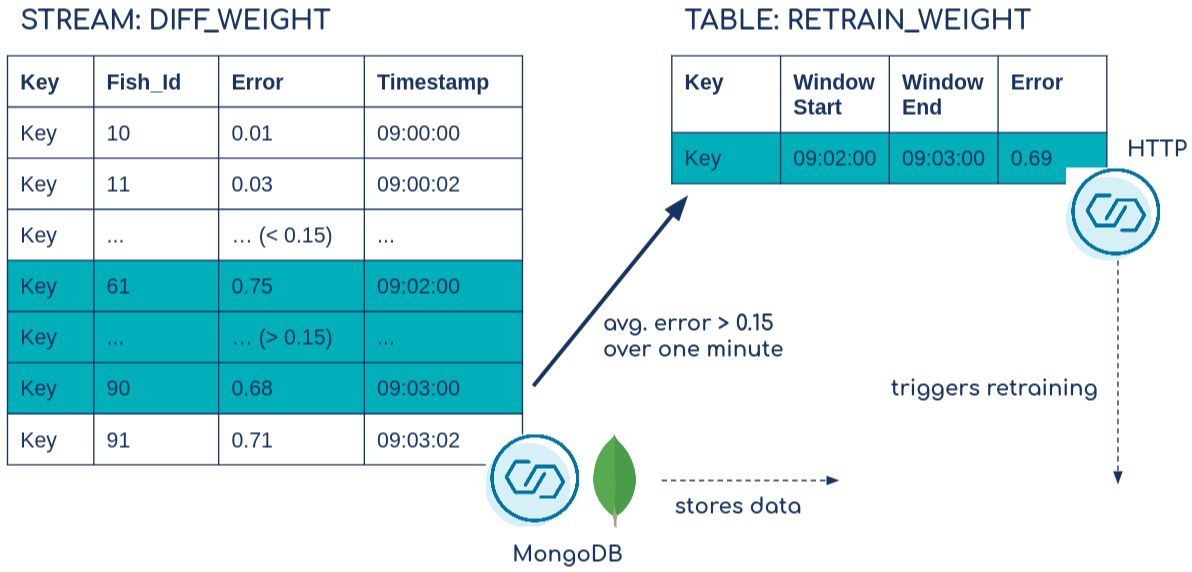
The following is a simplified representation (does not contain all columns) of the joined stream DIFF_WEIGHT and table RETRAIN_WEIGHT behaviour in combination with the Kafka Connect connectors:
Set up and run
Prerequisites: Docker, Docker Compose
With docker-compose up -d, we start all containers:
- ZooKeeper
- Kafka broker (for more information about its configurations, see the documentation)
- KAFKA_AUTO_CREATE_TOPICS_ENABLE: “true” ensures that we do not need to manually create the Kafka topic in which the producer sends its messages
- We also run a Bash command that automatically creates the topics weight-train and weight-diff (for the connectors) once the broker is ready
- Kafka Connect (for more information about its configurations, see the documentation)
- Note: Both the MongoDB Sink Connector and the HTTP Sink Connector are not part of the default connectors; therefore, we download it from Confluent Hub and run it with a Bash command
- ksqlDB server and ksqlDB client
- MongoDB
- Kafka producer
- A Docker image built to execute the fat JAR that continuously produces fake data into two topics: machine-measurement and machine-weight
- Kafka Streams
- A Docker image built to execute the fat JAR that predicts the weight on real-time data
- RStudio
- A Docker image built to provide an API with the prediction functions as well as retraining function
We need to wait some time until the Kafka broker is fully up and running. Then, we start both connectors with the commands:
curl -X POST -H "Content-Type: application/json" --data @MongoDBConnector.json http://localhost:8083/connectors | jq
curl -X POST -H "Content-Type: application/json" --data @HTTPConnector.json http://localhost:8083/connectors | jq
We also run ksqlDB client with the command:
docker exec -it ksqldb-cli ksql http://ksqldb-server:8088
And we create the streams and the table, and take a look at the data flow with the command:
SELECT * FROM DIFF_WEIGHT EMIT CHANGES;
The Error column displays the prediction error. For the first 60 fish (species of salmon) the error is very small so that the model predicts the fish weight very well. After that, the process changes, and starting with Fish_Id 61 a new species, walleye, is processed. Since the model is only trained with salmon fish and the relationship between size and weight differ for walleye fish, the model prediction results decrease dramatically.
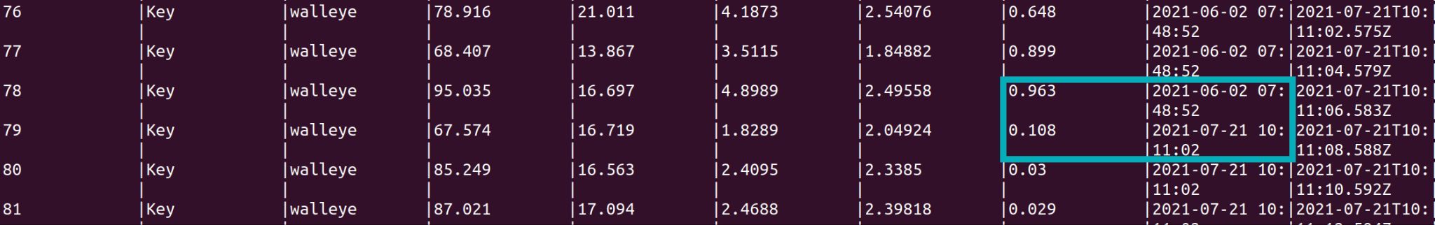
We continue looking at the stream and see that after some time the prediction results increase again and the model time (the time the model was trained) also changes. That is the moment when the retraining process is applied and a new model is now running on the real-time data.
After 60 walleye fish, salmon is produced again. However, the model takes the species into account when it is retrained, so the new model can deal with both species and the prediction results remain accurate.
Finally, we want to gain more insights into the retraining trigger.
SET 'auto.offset.reset'='earliest';
SELECT * FROM RETRAIN_WEIGHT EMIT CHANGES;

The average error was around 41% for one minute. This error emitted the event, triggered the HTTP Sink Connector, and consequently started the retraining process.
Note, when executing this tutorial the values might change because of a different start and end of the time window.
Data pipeline insights
To understand how the pipeline performs, we inspect the error (predicted weight versus real weight) over the events.
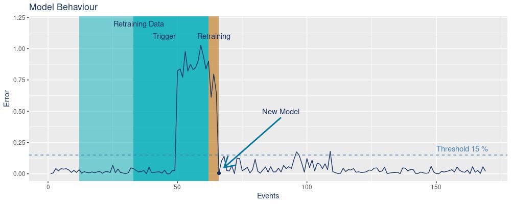
We see on the x-axis the number of events and on the y-axis the error. First, salmon is processed and the error stays low (under the threshold of 15%). Once walleye comes into play the error increases because the model is not trained with that data. The Trigger period defines the time frame in which the error exceeds the threshold on average over one minute. We start the retraining process with the last 50 data points (blue Retraining Data box). This period includes walleye as well as salmon. The time needed for the actual retraining is displayed in the orange Retraining box. In this period the data is requested, the model is retrained, and finally saved.
Once the new model is applied, we see that the prediction error decreases again.
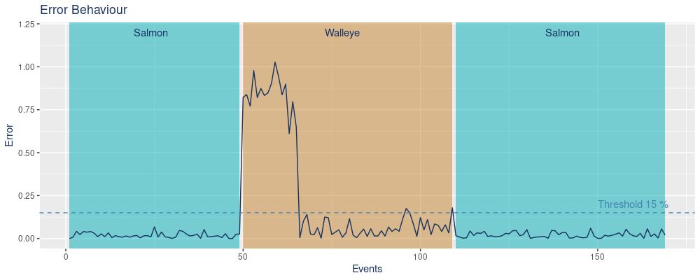
Here again, we highlight the error concerning the fish species. As previously explained, the model underperforms once walleye is processed. However, the retrained model performs well for both species which can be observed when salmon is again processed but the error remains low.
Even though the pipeline works as expected, there are some limitations that have to be considered.
First, all Kafka topics in this example only have a single partition, which can obviously not be a general assumption. Multi-partitioned topics are a common characteristic of Kafka because they ensure scalability and Kafka Streams automatically parallelize the workload into several tasks in that case. More about the architecture of Kafka Streams can be found in the documentation. Unfortunately, R, and consequently plumber, is mono-thread which means it can not handle parallel requests. There are solutions to deal with this issue including those addressed in the article How to do an efficient R API? by Jean-Baptiste Pleynet. In an upcoming blog post, the focus will be on the data pipeline performance, especially on high data throughput and its resulting limitations, and will include possible solutions.
Finally, security is an important feature. In this tutorial, Kafka and all related services are running without authentication (except MongoDB) because this pipeline serves simply as an example. For production use cases, it is worth thinking about authentication when creating such a pipeline. You can find more information about authentication for Kafka in its documentation.
Conclusion
In this tutorial, we implemented a data pipeline for real-time prediction as well as retraining with Apache Kafka and R, mainly using Kafka Streams, ksqlDB, Kafka Connect, and the plumber package.
If you have problems when executing the tutorial or have any questions, feel free to reach out in the Community Forum or Slack.
Ist dieser Blog-Beitrag interessant? Jetzt teilen
Confluent-Blog abonnieren


