Apache Kafka®️ 비용 절감 방법 및 최적의 비용 설계 안내 웨비나 | 자세히 알아보려면 지금 등록하세요
ATM Fraud Detection with Apache Kafka and KSQL
Fraud detection is a topic applicable to many industries, including banking and financial sectors, insurance, government agencies and law enforcement and more. Fraud attempts have seen a drastic increase in recent years, making fraud detection more important than ever. Despite efforts on the part of the affected institutions, hundreds of millions of dollars are lost to fraud every year. Since relatively few cases show fraud in a large population, finding these can be tricky.
In banking, fraud can involve using stolen credit cards, forging checks, misleading accounting practices, etc. In insurance, 25% of claims contain some form of fraud, resulting in approximately 10% of insurance payout dollars. Fraud can range from exaggerated losses to deliberately causing an accident for the payout. With all the different methods of fraud, finding it becomes harder still.
Detecting fraudulent transactions is one of the classic use cases for real-time data. The business value is clear:
- Reduce exposure to risk by identifying fraud sooner in order to take action to stop it
- Improve customer experience by reducing false positives
Traditionally, fraud detection has been done using stream processing applications written in languages such as Java. Maybe it’s been done using Kafka Streams or Spark Streaming, too, but regardless of the framework, it has always required a strong understanding of the core language first. This reduces the base of developers who can access stream processing. KSQL changes this, because anyone who can write SQL can now write stream processing applications.
KSQL is a continuous query language. Whilst you can use it for interactive exploration of data—as we will see in a moment—its core purpose is building stream processing applications. Because KSQL is built on Kafka Streams, which is built on Apache Kafka®, it benefits from the horizontal scalability characteristics for both resilience and throughput.
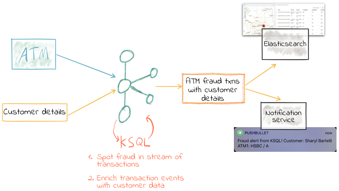
We’re going to see how we can take a stream of inbound ATM transactions and easily set up an application to detect transactions that look fraudulent. We’ll use a three key factors to determine if we think a transaction is fraudulent:
- The same account number as a previous transaction…
- …but at a different location
- …less than 10 minutes after the previous one
As part of the processing, we’ll also calculate the distance (as the crow flies) between the two suspect transactions, the time between them and, thus, how fast someone would have had to travel to plausibly make the transaction. This could feed into a second iteration of processing to refine the detection further.

We’re going to use Elasticsearch to store the transactions and enriched data, and Kibana to provide visualization and further data inspection capabilities.
Streams of ATM transactions
KSQL has supported joining between two streams of events since Confluent Platform 5.0. This means you can take two Kafka topics and join between them on a common key. This could be something like a stream of order events and a stream of shipment events—with a stream-stream join, you can match up orders being placed to those being shipped.
A stream-stream join can also make sense when done against the same stream of data, and that’s how we’re going to use it here. To start with, we’re going to take a simplified stream of ATM transactions and use it to understand what a stream-stream join is doing, and the semantics around it. Once we’ve done that, we’ll dive into a full-blown example with a data generator and some realistic test data.
I’m using Docker Compose to easily provision a test environment—if you want to follow along, you can find all the example files on GitHub.
Below are three transactions on three different accounts (ac_01, ac_02, ac_03). They have a transaction amount and location (both name and coordinates).
{"account_id": "ac_01", "atm": "ID_2276369282", "amount": 20, "location": {"lat": "38.6956033", "lon": "-121.5922283"}, "transaction_id": "01"}
{"account_id": "ac_02", "atm": "Flying Pig Bistro", "amount": 400, "location": {"lat": "37.766319", "lon": "-122.417422"}, "transaction_id": "02"}
{"account_id": "ac_03", "atm": "Wells Fargo", "amount": 50, "location": {"lat": "37.5522855", "lon": "-121.9797997"}, "transaction_id": "04"}
Let’s pull this into KSQL and see what we can do…
ksql> SET 'auto.offset.reset'='earliest';
ksql> CREATE STREAM ATM_TXNS (\
        account_id VARCHAR, \
        atm VARCHAR, \
        location STRUCT<lon DOUBLE,  \
                           lat DOUBLE>, \
        amount INT, \
        transaction_id VARCHAR) \
    WITH (\
        KAFKA_TOPIC='atm_txns', \
        VALUE_FORMAT='JSON');
ksql> SELECT ACCOUNT_ID, TRANSACTION_ID, AMOUNT, ATM FROM ATM_TXNS;
ac_01 | 01 | 20 | ID_2276369282
ac_02 | 02 | 400 | Flying Pig Bistro
ac_03 | 04 | 50 | Wells Fargo
So far, so good. No naughty transactions—just three regular ones from three different accounts. Now, let’s fire in two more. The first is a second transaction at the same location for the same account (someone forgot to pick up the drinks bill!); the second one is our nefarious fraudster, with a clone of the card for account ac_03 drawing cash from an ATM elsewhere:
{"account_id": "ac_02", "atm": "Flying Pig Bistro", "amount": 40, "location": {"lat": "37.766319", "lon": "-122.417422"}, "transaction_id": "03"}
{"account_id": "ac_03", "atm": "Barclays", "amount": 500, "location": {"lat": "33.5522855", "lon": "-120.9797997"}, "transaction_id": "X05"}
You’ll see these two new transactions appear straightaway in the KSQL output:
ksql> SELECT ACCOUNT_ID, TRANSACTION_ID, AMOUNT, ATM FROM ATM_TXNS;
ac_01 | 01 | 20 | ID_2276369282
ac_02 | 02 | 400 | Flying Pig Bistro
ac_03 | 04 | 50 | Wells Fargo
ac_02 | 03 | 40 | Flying Pig Bistro
ac_03 | X05 | 500 | Barclays
ac_03 is the one we’re interested in, and the transaction ID has an X prefix to help us spot it in the output, and the key thing is that it’s the same account in a different location (Flying Pig Bistro and then Barclays). What about time window? I’m glad you asked!
All Kafka messages have a timestamp (as well as a key and value). This can be set by the producing application, or it will otherwise take the value of the time at which the message arrived at the broker. KSQL exposes the message’s timestamp through the system column ROWTIME:
ksql> SELECT TIMESTAMPTOSTRING(ROWTIME, 'yyyy-MM-dd HH:mm:ss'),ACCOUNT_ID, TRANSACTION_ID, AMOUNT, ATM FROM ATM_TXNS;
2018-10-05 16:56:08 | ac_01 | 01 | 20 | ID_2276369282
2018-10-05 16:56:08 | ac_02 | 02 | 400 | Flying Pig Bistro
2018-10-05 16:56:08 | ac_03 | 04 | 50 | Wells Fargo
2018-10-05 17:01:59 | ac_02 | 03 | 40 | Flying Pig Bistro
2018-10-05 17:01:59 | ac_03 | X05 | 500 | Barclays
The two transactions for account ac_03 occurred within the span of just over five minutes.
By eyeballing this data, we can spot that something doesn’t look right; but how do we express this in stream processing terms? Enter stream-stream joins.
Join the streams (but don’t cross them)
Just as rows from two database tables can be joined, the same is possible with streams. The only difference is that since streams are unbounded (semantically—and often in practice—there is no defined end to the events arriving on the stream), the join syntax needs to account for this. Whilst a join between two tables in a database will consider all rows as candidates for matching on the join key, a stream-stream join will typically expect a window in which to look for events—which are, in effect, “rows”—to join. Otherwise, the stream processing engine would have to cache all events indefinitely.
In KSQL, the time window is expressed using the WITHIN clause of the join. You can specify either a single window value which applies to either side of the event, or two window values, giving the range before and after the event in which the join is to be evaluated. This time window is a convenient vehicle for our fraud criteria—any two transactions within a 10-minute window are to be captured.
We’ll begin by creating a second KSQL stream for the transaction events:
CREATE STREAM ATM_TXNS_02 WITH (PARTITIONS=1) AS SELECT * FROM ATM_TXNS;
Now we have two identical streams, one of which is actually a clone of the first:
ksql> SHOW STREAMS;
Stream Name | Kafka Topic | Format
ATM_TXNS | atm_txns | JSON ATM_TXNS_02 | ATM_TXNS_02 | JSON
ksql> SELECT TIMESTAMPTOSTRING(ROWTIME, 'yyyy-MM-dd HH:mm:ss'), ACCOUNT_ID, TRANSACTION_ID, AMOUNT, ATM FROM ATM_TXNS_02; 2018-10-05 16:56:08 | ac_03 | 04 | 50 | Wells Fargo 2018-10-05 16:56:08 | ac_01 | 01 | 20 | ID_2276369282 2018-10-05 17:01:59 | ac_03 | X05 | 500 | Barclays 2018-10-05 16:56:08 | ac_02 | 02 | 400 | Flying Pig Bistro 2018-10-05 17:01:59 | ac_02 | 03 | 40 | Flying Pig Bistro
Note: This is a necessary step that in principle could be handled by KSQL. It is tracked in GitHub issue 2030.
ksql> SELECT TIMESTAMPTOSTRING(T1.ROWTIME, 'yyyy-MM-dd HH:mm:ss'), TIMESTAMPTOSTRING(T2.ROWTIME, 'yyyy-MM-dd HH:mm:ss'), \
             T1.ACCOUNT_ID, T2.ACCOUNT_ID, \
             T1.TRANSACTION_ID, T2.TRANSACTION_ID, \
             T1.LOCATION, T2.LOCATION \
      FROM   ATM_TXNS T1 \
      INNER JOIN ATM_TXNS_02 T2 \
                 WITHIN 10 MINUTES \
                 ON T1.ACCOUNT_ID = T2.ACCOUNT_ID ;
2018-10-05 16:56:08 | 2018-10-05 16:56:08 | ac_01 | ac_01 | 01 | 01 | {LON=-121.5922283, LAT=38.6956033} | {LON=-121.5922283, LAT=38.6956033}
2018-10-05 16:56:08 | 2018-10-05 16:56:08 | ac_02 | ac_02 | 02 | 02 | {LON=-122.417422, LAT=37.766319} | {LON=-122.417422, LAT=37.766319}
2018-10-05 16:56:08 | 2018-10-05 17:01:59 | ac_02 | ac_02 | 02 | 03 | {LON=-122.417422, LAT=37.766319} | {LON=-122.417422, LAT=37.766319}
2018-10-05 16:56:08 | 2018-10-05 16:56:08 | ac_03 | ac_03 | 04 | 04 | {LON=-121.9797997, LAT=37.5522855} | {LON=-121.9797997, LAT=37.5522855}
2018-10-05 16:56:08 | 2018-10-05 17:01:59 | ac_03 | ac_03 | 04 | X05 | {LON=-121.9797997, LAT=37.5522855} | {LON=-120.9797997, LAT=33.5522855}
2018-10-05 17:01:59 | 2018-10-05 16:56:08 | ac_02 | ac_02 | 03 | 02 | {LON=-122.417422, LAT=37.766319} | {LON=-122.417422, LAT=37.766319}
2018-10-05 17:01:59 | 2018-10-05 17:01:59 | ac_02 | ac_02 | 03 | 03 | {LON=-122.417422, LAT=37.766319} | {LON=-122.417422, LAT=37.766319}
2018-10-05 17:01:59 | 2018-10-05 16:56:08 | ac_03 | ac_03 | X05 | 04 | {LON=-120.9797997, LAT=33.5522855} | {LON=-121.9797997, LAT=37.5522855}
2018-10-05 17:01:59 | 2018-10-05 17:01:59 | ac_03 | ac_03 | X05 | X05 | {LON=-120.9797997, LAT=33.5522855} | {LON=-120.9797997, LAT=33.5522855}
Looking at the output, we see a lot more than just the fraudulent transaction we’re expecting to identify. We can explain these additional matches as thus:
| Commentary | T1 timestamp |
T2 timestamp |
T1 account |
T2 account |
T1 TXN ID |
T2 TXN ID |
T1 Location |
T2 Location |
| self-join | 2018-10-05 16:56:08 | 2018-10-05 16:56:08 | ac_01 | ac_01 | 01 | 01 | {LON=-121.5922283, LAT=38.6956033} | {LON=-121.5922283, LAT=38.6956033} |
| self-join | 2018-10-05 16:56:08 | 2018-10-05 16:56:08 | ac_02 | ac_02 | 02 | 02 | {LON=-122.417422, LAT=37.766319} | {LON=-122.417422, LAT=37.766319} |
| self-join | 2018-10-05 16:56:08 | 2018-10-05 17:01:59 | ac_02 | ac_02 | 02 | 03 | {LON=-122.417422, LAT=37.766319} | {LON=-122.417422, LAT=37.766319} |
| self-join | 2018-10-05 16:56:08 | 2018-10-05 16:56:08 | ac_03 | ac_03 | 04 | 04 | {LON=-121.9797997, LAT=37.5522855} | {LON=-121.9797997, LAT=37.5522855} |
| !FRAUD! | 2018-10-05 16:56:08 | 2018-10-05 17:01:59 | ac_03 | ac_03 | 04 | X05 | {LON=-121.9797997, LAT=37.5522855} | {LON=-120.9797997, LAT=33.5522855} |
| valid (same location, not shown) | 2018-10-05 17:01:59 | 2018-10-05 16:56:08 | ac_02 | ac_02 | 03 | 02 | {LON=-122.417422, LAT=37.766319} | {LON=-122.417422, LAT=37.766319} |
| self-join | 2018-10-05 17:01:59 | 2018-10-05 17:01:59 | ac_02 | ac_02 | 03 | 03 | {LON=-122.417422, LAT=37.766319} | {LON=-122.417422, LAT=37.766319} |
| !FRAUD! (duplicate) | 2018-10-05 17:01:59 | 2018-10-05 16:56:08 | ac_03 | ac_03 | X05 | 04 | {LON=-120.9797997, LAT=33.5522855} | {LON=-121.9797997, LAT=37.5522855} |
| self-join | 2018-10-05 17:01:59 | 2018-10-05 17:01:59 | ac_03 |
ac_03X05X05{LON=-120.9797997, LAT=33.5522855}{LON=-120.9797997, LAT=33.5522855}
The first thing to do is weed out the join results where it’s just the same event joining to itself (that is, the transaction ID is the same):
ksql> SELECT
      […]
      WHERE T1.TRANSACTION_ID != T2.TRANSACTION_ID ;
2018-10-05 17:01:59 | 2018-10-05 16:56:08 | ac_02 | ac_02 | 03 | 02 | {LON=-122.417422, LAT=37.766319} | {LON=-122.417422, LAT=37.766319}
2018-10-05 17:01:59 | 2018-10-05 16:56:08 | ac_03 | ac_03 | X05 | 04 | {LON=-120.9797997, LAT=33.5522855} | {LON=-121.9797997, LAT=37.5522855}
2018-10-05 16:56:08 | 2018-10-05 17:01:59 | ac_02 | ac_02 | 02 | 03 | {LON=-122.417422, LAT=37.766319} | {LON=-122.417422, LAT=37.766319}
2018-10-05 16:56:08 | 2018-10-05 17:01:59 | ac_03 | ac_03 | 04 | X05 | {LON=-121.9797997, LAT=37.5522855} | {LON=-120.9797997, LAT=33.5522855}
Much better. Now, we just need to eliminate the transactions on the same account that took place at the same location—in this model, our fraud criteria determine those as unsuspicious.
ksql> SELECT
      […]
      WHERE
      […]
      (T1.location->lat != T2.location->lat OR \
       T1.location->lon != T2.location->lon);
2018-10-05 16:56:08 | 2018-10-05 17:01:59 | ac_03 | ac_03 | 04 | X05 | {LON=-121.9797997, LAT=37.5522855} | {LON=-120.9797997, LAT=33.5522855}
2018-10-05 17:01:59 | 2018-10-05 16:56:08 | ac_03 | ac_03 | X05 | 04 | {LON=-120.9797997, LAT=33.5522855} | {LON=-121.9797997, LAT=37.5522855}
The only two results are those on the account ac_03, one being genuine (transaction ID 04) and the other fraudulent (X05). We’re getting both returned, as each is an event on the left hand stream (the driving one) that joins to the other based on the time window specified (10 minutes before or after the driving event). All we need to do is change our join window to only return events that happen after the one we’re using to drive the join. To do this, simply specify a zero BEFORE threshold in the WITHIN criteria:
ksql> SELECT
      […]
      WITHIN (0 MINUTES, 10 MINUTES) \
      […]
2018-10-05 16:56:08 | 2018-10-05 17:01:59 | ac_03 | ac_03 | 04 | X05 | {LON=-121.9797997, LAT=37.5522855} | {LON=-120.9797997, LAT=33.5522855}
With the core logic of the statement built, let’s add in a few more bells and whistles. Using the built-in GEO_DISTANCE function, we can include a column in the output showing the distance between the two transactions:
ksql> SELECT
      […]
      T1.location, \
      T2.location, \
      GEO_DISTANCE(T1.location->lat, T1.location->lon, T2.location->lat, T2.location->lon, 'KM') AS DISTANCE_BETWEEN_TXN_KM, \
      […]
{LON=-121.9797997, LAT=37.5522855} | {LON=-120.9797997, LAT=33.5522855} | 453.87740037465375
We see that transaction 04 took place over 450 kilometers, as the crow flies from X05. What was the time duration between them? We can answer this pretty easily based on the timestamp, but it’s more sensible just to include it in the query:
ksql> SELECT
        […]
        (T2.ROWTIME - T1.ROWTIME) AS MILLISECONDS_DIFFERENCE,  \
        (CAST(T2.ROWTIME AS DOUBLE) - CAST(T1.ROWTIME AS DOUBLE)) / 1000 / 60 AS MINUTES_DIFFERENCE,  \
        (CAST(T2.ROWTIME AS DOUBLE) - CAST(T1.ROWTIME AS DOUBLE)) / 1000 / 60 / 60 AS HOURS_DIFFERENCE,  \
        GEO_DISTANCE(T1.location->lat, T1.location->lon, T2.location->lat, T2.location->lon, 'KM') / ((CAST(T2.ROWTIME AS DOUBLE) - CAST(T1.ROWTIME AS DOUBLE)) / 1000 / 60 / 60) AS KMH_REQUIRED,
        […]
351473 | 5.8578833333333336 | 0.09763138888888889 | 4648.888083433872
We’ve also combined the distance and time calculations to derive the speed at which someone would have to move between the two events. At 4,648 kph, it’s almost four times the speed of the fastest supersonic car—we can be pretty sure it’s fraudulent!
One remaining point to make about the above query is that the message’s timestamp (ROWTIME) is cast from its BIGINT data type to DOUBLE so that the subsequent division arithmetic will work.
Running it with “real” data
To see what our query looks like against a continuous stream of transactions, let’s fire up our data generator. I’m using an open source tool called gess, which I’ve forked and tweaked to suit this demo.
It works by taking a list of ATMs, generating transactions against them and emitting these to UDP. UDP is a networking protocol in the same way that TCP is, but unlike TCP, UDP doesn’t require any kind of acknowledgement of delivery. Instead, it just fires bytes out into the ether, and if someone picks them up, that’s great, and if not, that’s fine too. It makes for a useful test rig where we can start up the data generator and simply tap into the event stream as and when we want to.
To route the events to Kafka from UDP, I’m using two great little command line tools that any self-respecting engineer should know: netcat (nc) and kafkacat. Netcat listens for the UDP traffic, which is then piped to kafkacat. kafkacat simply takes any input from stdin and sends it as messages to the target topic.
Here’s netcat picking up the events:
$ nc -v -u -l 6900
{"account_id": "a9", "timestamp": "2018-10-07T20:40:48.585666", "atm": "ATM : 3616415159", "amount": 50, "location": {"lat": "53.8233994", "lon": "-1.4865327"}, "transaction_id": "e406bf57-ca68-11e8-a4cb-186590d22a35"}
{"account_id": "a102", "timestamp": "2018-10-07T20:40:49.087221", "atm": "Co-op Bank", "amount": 400, "location": {"lat": "53.7986913", "lon": "-1.2518281"}, "transaction_id": "e4534754-ca68-11e8-a119-186590d22a35"}
{"account_id": "a496", "timestamp": "2018-10-07T20:40:49.589651", "atm": "Link", "amount": 50, "location": {"lat": "53.8442149", "lon": "-1.5094248"}, "transaction_id": "e49ff142-ca68-11e8-9c4f-186590d22a35"}
{"account_id": "a223", "timestamp": "2018-10-07T20:40:50.093244", "atm": "ATM : 5523013160", "amount": 400, "location": {"lat": "53.6781485", "lon": "-1.4991026"}, "transaction_id": "e4ecc8fd-ca68-11e8-9132-186590d22a35"}
[...]
Here’s netcat piping it to a Kafka topic:
$ nc -v -u -l 6900 | \
    docker run --interactive --rm --network ksql-atm-fraud-detection_default confluentinc/cp-kafkacat \
    kafkacat -b kafka:29092 -P -t atm_txns_gess
Note that there’s no console output from this, because it’s being redirected to kafkacat.
Event time processing with KSQL
We need to make one change to the KSQL statement that we developed above. Whereas we were previously using the Kafka message timestamp as the event rowtime, now, we want to use the timestamp field that’s included in the payload of the message. This is easy to do with KSQL by simply specifying the TIMESTAMP field in the WITH clause:
CREATE STREAM ATM_TXNS_GESS (\
              account_id     VARCHAR, \
              atm            VARCHAR, \
              location       STRUCT<lon DOUBLE,  \
                                    lat DOUBLE>, \
              amount         INT, \
              timestamp      VARCHAR, \
              transaction_id VARCHAR) \
         WITH (\
              KAFKA_TOPIC='atm_txns_gess', \
              VALUE_FORMAT='JSON', \
              TIMESTAMP='timestamp', \
              TIMESTAMP_FORMAT='yyyy-MM-dd HH:mm:ss X');
Just to check that KSQL is indeed picking up the value of timestamp field in the source message, let’s run a query to report the timestamp field’s value along with the system column ROWTIME, which represents the timestamp with which KSQL will process the message:
ksql> SELECT TIMESTAMPTOSTRING(ROWTIME, 'yyyy-MM-dd HH:mm:ss Z'), timestamp FROM ATM_TXNS_GESS;
2018-10-07 22:31:39 +0000 | 2018-10-07 22:31:39 +0000
2018-10-07 22:31:40 +0000 | 2018-10-07 22:31:40 +0000
2018-10-07 22:26:58 +0000 | 2018-10-07 22:26:58 +0000
2018-10-07 22:31:41 +0000 | 2018-10-07 22:31:41 +0000
As expected, they match. One subtlety to notice here is that the third message above is dated earlier than the one previously. That’s because the ATM transactions may be arriving out of order. However, KSQL will process them based on event time (i.e., timestamp value in the source message, when the actual ATM transaction occurred) rather than processing time, which refers to when the message arrived at the system.
Bringing together our new source stream (ATM_TXNS_GESS) with the logic we prototyped above gives us this code to run:
CREATE STREAM ATM_TXNS_GESS_02 WITH (PARTITIONS=1) AS SELECT * FROM ATM_TXNS_GESS;CREATE STREAM ATM_POSSIBLE_FRAUD
WITH (PARTITIONS=1) AS
SELECT T1.ROWTIME AS T1_TIMESTAMP, T2.ROWTIME AS T2_TIMESTAMP,
GEO_DISTANCE(T1.location->lat, T1.location->lon, T2.location->lat, T2.location->lon, 'KM') AS DISTANCE_BETWEEN_TXN_KM,
(T2.ROWTIME - T1.ROWTIME) AS MILLISECONDS_DIFFERENCE,
(CAST(T2.ROWTIME AS DOUBLE) - CAST(T1.ROWTIME AS DOUBLE)) / 1000 / 60 AS MINUTES_DIFFERENCE,
GEO_DISTANCE(T1.location->lat, T1.location->lon, T2.location->lat, T2.location->lon, 'KM') / ((CAST(T2.ROWTIME AS DOUBLE) - CAST(T1.ROWTIME AS DOUBLE)) / 1000 / 60 / 60) AS KMH_REQUIRED,
T1.ACCOUNT_ID AS ACCOUNT_ID,
T1.TRANSACTION_ID, T2.TRANSACTION_ID,
T1.AMOUNT, T2.AMOUNT,
T1.ATM, T2.ATM,
CAST(T1.location->lat AS STRING) + ',' + CAST(T1.location->lon AS STRING) AS T1_LOCATION,
CAST(T2.location->lat AS STRING) + ',' + CAST(T2.location->lon AS STRING) AS T2_LOCATION
FROM ATM_TXNS_GESS T1
INNER JOIN ATM_TXNS_GESS_02 T2
WITHIN (0 MINUTES, 10 MINUTES)
ON T1.ACCOUNT_ID = T2.ACCOUNT_ID
WHERE T1.TRANSACTION_ID != T2.TRANSACTION_ID
AND (T1.location->lat != T2.location->lat OR
T1.location->lon != T2.location->lon)
AND T2.ROWTIME != T1.ROWTIME;
Checking the output shows that there are plenty of fraudulent transactions being detected:
SELECT T1_ACCOUNT_ID, \
       TIMESTAMPTOSTRING(T1_TIMESTAMP, 'yyyy-MM-dd HH:mm:ss'), TIMESTAMPTOSTRING(T2_TIMESTAMP, 'HH:mm:ss'), \
       T1_ATM, T2_ATM, \
       DISTANCE_BETWEEN_TXN_KM, MINUTES_DIFFERENCE \
FROM ATM_POSSIBLE_FRAUD;
a739 | 2018-10-08 15:35:58 | 15:38:31 | Halifax | Barclays Bank PLC | 15.698597512981406 | 2.55
a649 | 2018-10-08 15:36:22 | 15:38:04 | Yorkshire Bank | Barclays Bank PLC | 23.179463348879413 | 1.7
[...]
The execution statistics shows that we’ve processed multiple messages. In other words, we’ve detected many possibly fraudulent transactions:
ksql> DESCRIBE EXTENDED ATM_POSSIBLE_FRAUD;[...] Kafka topic : ATM_POSSIBLE_FRAUD (partitions: 1, replication: 1) [...] Local runtime statistics
messages-per-sec: 0.85 total-messages: 324 last-message: 10/9/18 11:25:11 AM UTC [...]
There are some changes to note from the query that we iteratively built up at the beginning of this article. These are just to streamline and tidy it up, but the core logic is the same.
- Add CREATE STREAM … AS to tell KSQL to persist this as a streaming application, and populate the named stream as a Kafka topic with the results.
- Retain the timestamp as an epoch rather than the VARCHAR that we’ve been using for printing it in human-readable format.
- Only include one of the ACCOUNT_ID fields in the output since they are equal, as stated in the JOIN criteria.
- Remove the intermediate calculated columns of the time difference between the two transactions.
- Include the name of the ATM at which each transaction took place.
- Wrangle the source LOCATION column (a STRUCT by default) into a comma-separated STRING. This is necessary for being able to index it into Elasticsearch as a geopoint.
Kafka + Elastic = ❤️
Using the above KSQL application, we’ve got a Kafka topic being populated with suspect ATM transactions. We can query this from the command line in KSQL to inspect it, but at the end of the day, it’s just a Kafka topic. We can use this Kafka topic for multiple independent purposes, including:
- Drive a microservice—perhaps to trigger an alert or block on a particular card
- Stream the data to a store, such as Elasticsearch, for visualization and analysis in Kibana
Streaming data from Kafka to Elasticsearch is easy using Kafka Connect and the Elasticsearch connector. Check out the code on GitHub for full details, but in essence, it’s two scripts:
- A dynamic mapping template for the Elasticsearch indices so that things like geopoints and timestamps are set up correctly
- A Kafka Connect JSON configuration specifying the Kafka topics from which to stream data and the corresponding Elasticsearch indices to load
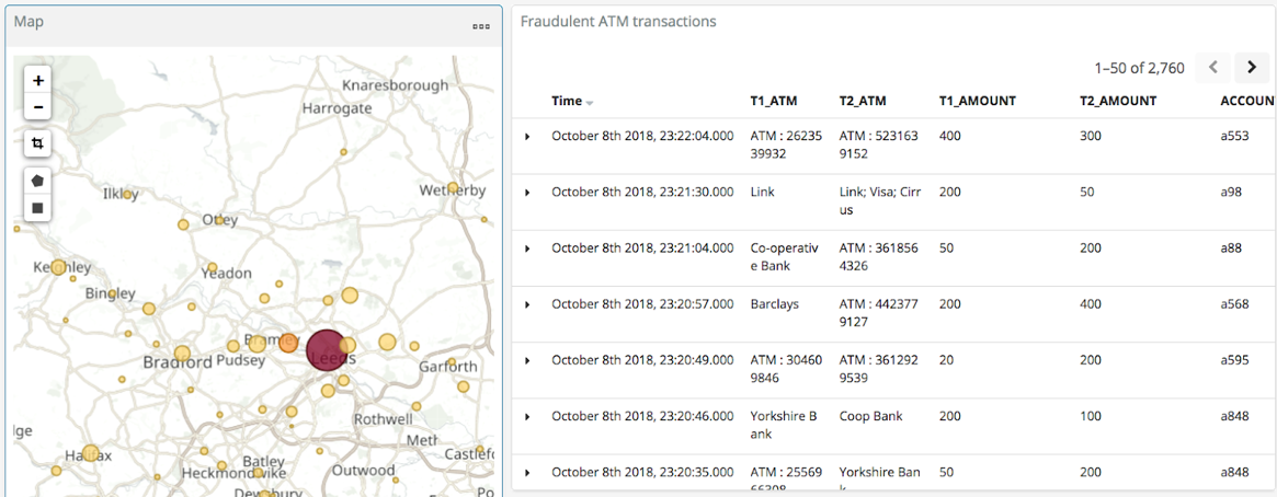
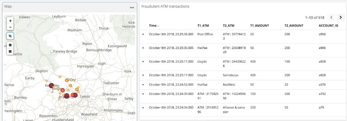
With the data in Elasticsearch, we can easily build some powerful dashboards and analyses with Kibana. Here’s a view of all suspected fraudulent activity in a region, with hotspots highlighted:
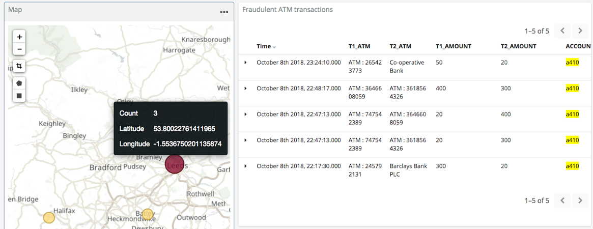
By selecting a specific account, all ATM transactions for that account can be shown for further analysis. Here, any fraud alerts for account a410 are shown and plotted on the map:
You can also use Kibana to draw a bounding box around a particular region of the map to filter events just for that area: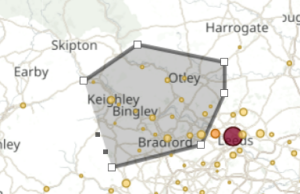
Enriching streams of events
We’ve taken an inbound stream of events and used KSQL to populate a Kafka topic of transactions that look potentially fraudulent. But all we have to go on is the account number. Wouldn’t it be more useful if we can include in our event stream information about the account itself? We can then show the account information in the visual analysis, as well as using it to drive notifications directly.
Let’s assume that we have all of our customer information in a database. Pretty standard place to keep it. It’s maintained by a separate application, and it is our master store of customer data. In this case I’m using MySQL, but it could be any RDBMS, really:
mysql> SELECT FIRST_NAME, LAST_NAME, EMAIL, ADDRESS FROM accounts WHERE ACCOUNT_ID='a42';
+------------+-----------+--------------------+------------------+
| FIRST_NAME | LAST_NAME | EMAIL              | ADDRESS          |
+------------+-----------+--------------------+------------------+
| Robin      | Moffatt   | robin@confluent.io | 22 Acacia Avenue |
+------------+-----------+--------------------+------------------+
1 row in set (0.00 sec)
Using Kafka Connect and a CDC tool such as Debezium, we can stream the contents of it to a Kafka topic, as well as any changes made to the data, in real time. With the data in a Kafka topic, it’s possible to model it as a table and join it to the event stream of ATM transactions:
ksql> SELECT FIRST_NAME, LAST_NAME, EMAIL, ADDRESS FROM accounts WHERE ACCOUNT_ID='a42';
Robin | Moffatt | robin@confluent.io | 22 Acacia Avenue
If something changes in the database, it’s reflected straight away in the Kafka topic (and thus KSQL table too):
So with an accurate mirror of the data from the table available in KSQL, it’s a simple matter to join this to the stream of ATM transactions:
ksql> SELECT A.ACCOUNT_ID, \
        C.FIRST_NAME + ' ' + C.LAST_NAME, \
        C.EMAIL, C.PHONE, \
        C.ADDRESS, \
        TIMESTAMPTOSTRING(A.T1_TIMESTAMP, 'yyyy-MM-dd HH:mm:ss'), TIMESTAMPTOSTRING(A.T2_TIMESTAMP, 'HH:mm:ss'), \
        A.T1_ATM, A.T2_ATM, \
        A.DISTANCE_BETWEEN_TXN_KM, A.MINUTES_DIFFERENCE \
FROM ATM_POSSIBLE_FRAUD A LEFT OUTER JOIN ACCOUNTS C ON A.ACCOUNT_ID = C.ACCOUNT_ID;
a279 | Shandeigh Isakovic | sisakovic5n@upenn.edu | +44 645 302 9358 | 49 Nevada Center | 2018-10-09 13:42:07 | 13:47:21 | Yorkshire Bank | ATM : 319429912 | 12.536338916950928 | 5.233333333333333
a769 | Kathe Cutteridge | kcutteridgehg@gov.uk | +44 501 421 3436 | 5 Jackson Pass | 2018-10-09 13:45:47 | 13:47:35 | Barclays | Co-Op | 14.448491852409132 | 1.8
[…]
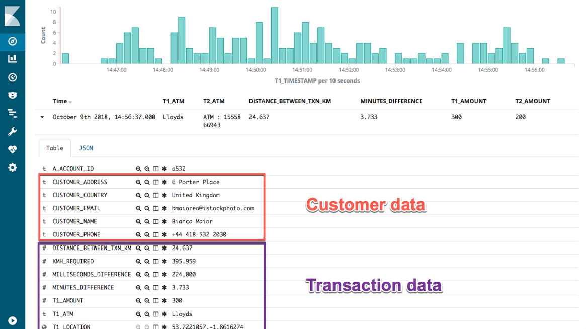
Persisting this as another new Kafka topic gives us a rich stream of events every time an ATM transaction occurs matching our fraud criteria. It also includes all the information we might want in order to contact the customer concerned:
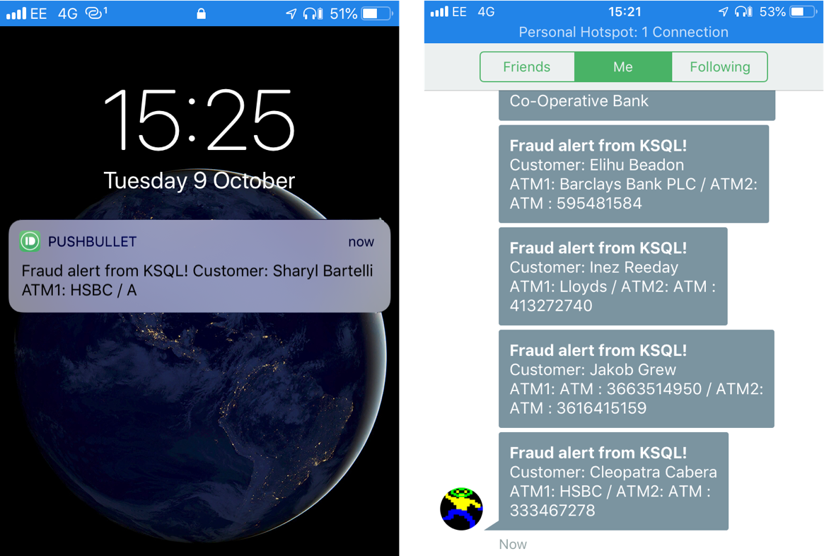
The same data is used for pushing fraud notifications to customers’ phones:
Conclusion
We’ve seen a few key concepts with KSQL:
- Detecting patterns in a stream of data based on an event’s time relative to another’s, as well as characteristics of the two events
- Populating a target Kafka topic with a real-time feed of these events matching the defined conditions
- Denormalizing data, bringing together events (facts) and additional information about entities within those (dimensions)
The enriched data from the Kafka topic, which is continually populated by KSQL, is streamed into Elasticsearch using Kafka Connect. From there, analysis and visualization are done in Kibana. This enriched topic serves as the driver for a microservice responsible for further actions based on suspected fraud on an account, such as putting a temporary hold on it or notifying the account holder.
Interested in more?
- Download Confluent Platform, the leading distribution of Apache Kafka
- Follow the example KSQL recipe based off this blog post, and try it at home!
- Learn about ksqlDB, the successor to KSQL, and see the latest syntax


